We have started a series of articles on tips and tricks for data scientists (mainly in Python and R). In case you have missed:
Python
1.How To Get The Mode From A List In Python
Assume that we have the following list:
mylist = [1,1,1,2,2,3,3]
and we want to get the mode, i.e. the most frequent element. We can use the following trick using the max and the lambda key.
max(mylist, key = mylist.count)
And we get 1 since this was the mode in our list. In case where there is a draw in the mode and you want to get the minimum or the maximum number, you can sort the list as follows:
mylist = [1,1,1,2,2,3,3,3]
max(sorted(mylist), key = mylist.count)
And we get 1
mylist = [1,1,1,2,2,3,3,3]
max(sorted(mylist, reverse=True), key = mylist.count)
And we get 3
In the above example, we had two modes, 1 and 3. By adding the sorted function we were able to get the min and the max respectively. Finally, this approach works with string elements too.
mylist = ['a','a','b','b','b']
max(mylist, key = mylist.count)
And we get ‘b’
2.How To Disable All Warnings In Python
You can disable all python warnings by running the following code block.
import sys
if not sys.warnoptions:
    import warnings
    warnings.simplefilter("ignore")
3.How to Copy Data And Paste Into A Pandas DataFrame
Firstly we need to copy the data-frame like data.
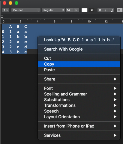
Then, run the following:
import pandas as pd
pd.read_clipboard()

4.How to Save Pandas Dataframes As Images
You can save Pandas Dataframes as images using the library dataframe-image. Then you can run:
import pandas as pd
import dataframe_image as dfi

df = pd.DataFrame({'A': [1,2,3,4],
                   'B':['A','B','C','D']})

dfi.export(df, 'dataframe.png')
Running the above, it will create a png image file with the dataframe as the image below.

5.How To Add A Progress Bar Into Pandas Apply
When we are applying a function to a big Data-Frame, we can’t see the progress of the function or an estimate on how long remains for the function to be applied to the whole dataset. We can solve this with the use of the tqdm library.
import pandas as pd
import numpy as np
from tqdm.notebook import tqdm
tqdm.pandas()

#dummy data
df=pd.DataFrame({"Value":np.random.normal(size=1500000)})
Let’s apply a simple function to our data but instead of using apply, we will use the progress_apply function.
df['Value'].progress_apply(lambda x: x**2)

R
6.Avoid Apply() Function In Large Datasets
When we are dealing with large datasets and there is a need to calculate some values like the row/column min/max/rank/mean etc we should avoid the apply function because it takes a lot of time. Instead, we can use the matrixStats package and its corresponding functions. Let’s provide some comparisons.
Example of Minimum value per Row
Assume that we want to get the minimum value of each row from a 500 x 500 matrix. Let’s compare the performance of the apply function from the base package versus the rowMins function from the matrixStats package.
library(matrixStats)
library(microbenchmark)
library(ggplot2)

x <- matrix( rnorm(5000 * 5000), ncol = 5000 )

tm <- microbenchmark(apply(x,1,min),
                     rowMins(x),
                     times = 100L
                    )

tm
And we get:
Unit: milliseconds
             expr      min         lq       mean    median        uq       max neval
 apply(x, 1, min) 981.6283 1034.98050 1078.04485 1065.4163 1107.9962 1327.9284   100
       rowMins(x)  42.1838   43.80065   46.55752   45.2255   47.6249   81.3097   100
As we can see from the output above, the apply function was 23 times slower than the rowMins. Below we represent the violin plot
autoplot(tm)

7.The Fastest Way To Read And Write Files In R
When we are dealing with large datasets, and we need to write many csv files or when the csv filethat we hand to read is huge, then the speed of the read and write command is important. We will compare the required time to write and read files of the following cases:
- base package
- data.table
- readr
Compare the Write times
We will work with a csv file of 1M rows and 10 columns which is approximately 180MB. Let’s create the sample data frame and write it to the hard disk. We will generate 10M observations from the Normal Distribution.
library(data.table)
library(readr)
library(microbenchmark)
library(ggplot2)

# create a 1M X 10 data frame

my_df<-data.frame(matrix(rnorm(1000000*10), 1000000,10))


# base
system.time({ write.csv(my_df, "base.csv", row.names=FALSE) })

# data.table
system.time({ fwrite(my_df, "datatable.csv") })

# readr
system.time({ write_csv(my_df, "readr.csv") })

As we can see from the elapsed time, the fwrite from the data.table is ~70 times faster than the base package and ~7times faster than the readr
Compare the Read Times
Let’s compare also the read times using the microbenchmark package.
tm <- microbenchmark(read.csv("datatable.csv"),
                     fread("datatable.csv"),
                     read_csv("datatable.csv"),
                     times = 10L
)

tm
autoplot(tm)

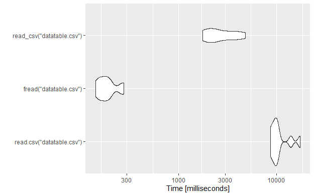
As we can see, again the fread from the data.table package is around 40 times faster than the base package and 8.5 times faster than the read_csv from the readr package. So, if you want to read and write files fastly then you should choose the data.table package.
8.How To Compare Objects In R

In 2020, the guru Hadley Wickham, built a new package called waldo for comparing complex R objects and making it easy to detect the key differences. You can find detailed examples in tidyverse.org as well as at the github. Let’s provide a simple example by comparing two data frames in R with waldo.
Compare 2 Data Frames in R
Let’s create the new data frames:
library(waldo)


df1<-data.frame(X=c(1,2,3), Y=c("a","b","c"), A=c(3,4,5))
df2<-data.frame(X=c(1,2,3,4), Y=c("A","b","c","d"), Z=c("k","l","m","n"), A=c("3","4","5","6"))
The df1:
  X Y A
1 1 a 3
2 2 b 4
3 3 c 5
And the df2:
  X Y Z A
1 1 A k 3
2 2 b l 4
3 3 c m 5
4 4 d n 6
Let’s compare them:
waldo::compare(df1,df2)
And we get:
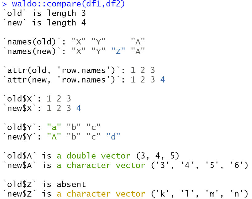
As we can see it captures all the differences and the output is in a friendly format of different colors depending on the difference. More particularly, it captures that:
- The df1 has 3 rows where df2 has 2
- The df2 has an extra column name and it shows where is the difference in the order.
- It shows the rows names and the differences
- It compares each column, X, Y, A, Z
- It detected the difference in the data type of column A where in the first is double and in the second is character
- It returns that there is a new column called Z.
9.How To Install And Load Packages Dynamically
When we share an R script file with someone else, we assumed that they have already installed the required R packages. However, this is not always the case and for that reason, I strongly suggest adding this piece of code to every shared R script which requires a package. Let’s assume that your code requires the following three packages: “readxl“, “dplyr“, “multcomp” .
The script below checks, if the package exists, and if not, then it installs it and finally it loads it to R
mypackages<-c("readxl", "dplyr", "multcomp")

for (p in mypackages){
  if(!require(p, character.only = TRUE)){
    install.packages(p)
    library(p, character.only = TRUE)
  }
  }
10.How To Convert All Character Variables To Factors
Let’s say that we want to convert all Character Variables to Factors and we are dealing with a large data frame of many columns which means that is not practical to convert them one by one. Thus, our approach is to detect the “char” variables and to convert them to “Factors”.
Let’s provide a toy example:
df<-data.frame(Gender = c("F", "F", "M","M","F"),
               Score  = c(80, 70, 65, 85, 95),
               Type = c("A","B","C","B","B"))
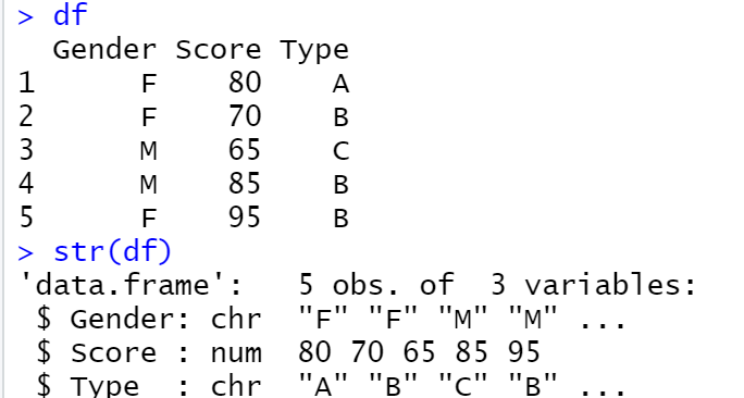
As we can see, the Gender and Type are char variables. Let’s convert them to factors.
df[sapply(df, is.character)] <- lapply(df[sapply(df, is.character)], as.factor)

As we can see, we managed to convert them. Now, you can also rename and relevel the factors. Notice that we could work in the other way around by converting the Factors to Characters. Generally, we can change different data types.



3 thoughts on “10 Tips And Tricks For Data Scientists Vol.6”
I think the easier, and probably more efficient way of converting character variables to factors is mutate_if in dplyr:
mutate_if(is.character, as.factor)
Yes I agree, I try to keep it simple without using libraries like dplyr.
I think the fastest way to read a file in R is using vroom package. It’s much faster than the fread and also memory efficient, as it doesn’t load all of the data into the env at once.