I have started a series of articles on tips and tricks for data scientists (mainly in Python and R). In case you missed vol 1 and vol 2.
Python
1. How to work with JSON cells in pandas
Assume that you are dealing with a pandas DataFrame where one of your columns is in JSON format and you want to extract specific information. For this example, we will work with the doc_report.csv dataset from Kaggle.
import pandas as pd
import ast
pd.set_option("max_colwidth", 180)
doc = pd.read_csv("doc_reports.csv", index_col=0)
# print the properties column
doc['properties']

If we look at the data, the properties field is in JSON format. This means that we need to convert it to a dictionary and then extract the required information. We will work with the ast library to convert it to a dictionary and then we will create separate columns for each key as follows:
dummy = doc['properties'].apply(lambda x: ast.literal_eval(x))
doc['gender'] = dummy.apply(lambda x:x.get('gender'))
doc['nationality'] = dummy.apply(lambda x:x.get('nationality'))
doc['document_type'] = dummy.apply(lambda x:x.get('document_type'))
doc['date_of_expiry'] = dummy.apply(lambda x:x.get('date_of_expiry'))
doc['issuing_country'] = dummy.apply(lambda x:x.get('issuing_country'))
# lets get the columns
doc[['gender', 'nationality', 'document_type', 'date_of_expiry','issuing_country' ]]

As you can see, we converted a JSON data type cell to columns based on the key values.
2. How to change multiple column values with applymap
We will provide an example of how you can change multiple column values in pandas DataFrames using the applymap function. Assume that your DataFrame takes values 1, 2, and 3 and you want to apply the following mapping function:
- If
1, then0. - If
2or3, then1.
df = pd.DataFrame({'A':[1,1,2,2,3,3],
'B':[1,2,3,1,2,3]})
df
        A	B
0	1	1
1	1	2
2	2	3
3	2	1
4	3	2
5	3	3
Using the applymap function:
# create the mapping dictionary
d = {1 : 0, 2: 1, 3: 1}
# apply it to all columns
df.applymap(d.get)
        A	B
0	0	0
1	0	1
2	1	1
3	1	0
4	1	1
5	1	1
3. How to build treemaps with Plotly
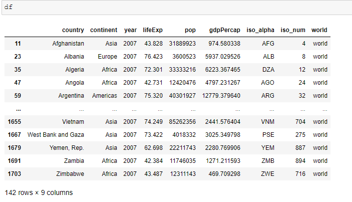
With plotly.express, you can easily create fancy treemaps. For example, let’s say that we want to represent the life expectancy by country taking into consideration the continent and the population of the country. So, in the treemap below, the size of the rectangle refers to the population and the color refers to the life expectancy. The higher the life expectancy, the bluer the color is. The lower the life expectancy, the redder the color is.
import plotly.express as px
import numpy as np
df = px.data.gapminder().query("year == 2007")
df["world"] = "world" # in order to have a single root node
fig = px.treemap(df, path=['world', 'continent', 'country'], values='pop',
                  color='lifeExp', hover_data=['iso_alpha'],
                  color_continuous_scale='RdBu',
                  color_continuous_midpoint=np.average(df['lifeExp'], weights=df['pop']))
fig.show()


4. How to get the correlation between two DataFrames
df1 = pd.DataFrame({'x11' : [10,20,30,40,50,55,60],
                    'x12' : [11,15,20,30,35,60,70]})
df2 = pd.DataFrame({'x21' : [100,150,200,250,300,400,500],
                    'x22' : [110,150,180,250,300,400,600]})
pd.concat([df1, df2], axis=1, keys=['df1', 'df2']).corr().loc['df1', 'df2']
    x21      x22
x11 0.953873 0.900050
x12 0.988908 0.975597
5. How to truncate dates to a month in pandas
Assume that you are dealing with the following DataFrame:
import pandas as pd
df = pd.DataFrame({'MyDate': ['2020-03-11', '2021-04-26', '2021-01-17']})
df['MyDate'] = pd.to_datetime(df.MyDate)
df
    MyDate
0   2020-03-11
1   2021-04-26
2   2021-01-17
And you want to truncate the date to a month:
df['Truncated'] = df['MyDate'] + pd.offsets.MonthBegin(-1)
# OR
# df['Truncated'] = df['MyDate'] - pd.offsets.MonthBegin(1)
df
  MyDate     Truncated
0 2020-03-11 2020-03-01
1 2021-04-26 2021-04-01
2 2021-01-17 2021-01-01
6. How to append multiple CSV files from a folder in pandas
Assume that you have multiple CSV files located in a specific folder and you want to concatenate all of them in a pandas DataFrame. We assume that our CSV files are under the My_Folder.
import os
import pandas as pd
# create an empty pandas data frame
df = pd.DataFrame()
# iterate over all files within "My_Folder"
for file in os.listdir("My_Folder"):
    if file.endswith(".csv"):
        df = pd.concat([df , pd.read_csv(os.path.join("My_Folder", file))], axis=0 )
# reset the index
df.reset_index(drop=True, inplace=True)
df
Now the df consists of the CSV files within My_Folder.
7. How to concatenate multiple CSV files in Python
Assume that you have multiple CSV files located in a specific folder and you want to concatenate all of them and save them to a file called merged.csv. We can work with pandas and use the trick with mode=a within the .to_csv(), which means append:
import os
import pandas as pd
# iterate over all files within "My_Folder"
for file in os.listdir("My_Folder"):
    if file.endswith(".csv"):
        tmp = pd.read_csv(os.path.join("My_Folder", file))
        tmp.to_csv("merged.csv", index=False, header=False, mode='a')
8. How to concatenate multiple TXT files in Python
Assume that you have multiple .txt files and you want to concatenate all of them into a unique .txt file. Assume that your .txt files are within the dataset folder. Then you will need to get their paths:
import os
# find all the txt files in the dataset folder
inputs = []
for file in os.listdir("dataset"):
    if file.endswith(".txt"):
        inputs.append(os.path.join("dataset", file))
# concatanate all txt files in a file called merged_file.txt
with open('merged_file.txt', 'w') as outfile:
    for fname in inputs:
        with open(fname, encoding="utf-8", errors='ignore') as infile:
            outfile.write(infile.read())
With the snippet above, we managed to concatenate all of them into one file called merged_file.txt. In the case where the files are large, you can work as follows:
with open('merged_file.txt', 'w') as outfile:
    for fname in inputs:
        with open(fname, encoding="utf-8", errors='ignore') as infile:
            for line in infile:
                outfile.write(line)
R
9. How to get the correlation between two DataFrames
Let’s see how we can get the column-wise correlation between two DataFrames in R:
df1 = data.frame(x11 = c(10,20,30,40,50,55,60),
                 x12 = c(11,15,20,30,35,60,70)
                 )
df2 = data.frame(x21 = c(100,150,200,250,300,400,500),
                 x22 = c(110,150,180,250,300,400,600)
                 )
cor(df1,df2)
    x21       x22
x11 0.9538727 0.9000503
x12 0.9889076 0.9755973
10. The “Count(Case When … Else … End)” in R
When I run queries in SQL (or even HiveQL, Spark SQL, and so on), it is quite common to use the count(case when.. else ... end) syntax. Today, I will provide you an example of how you run this type of command in dplyr. Let’s start:
library(sqldf)
library(dplyr)
df<-data.frame(id = 1:10,
               gender = c("m","m","m","f","f","f","m","f","f","f"),
               amt= c(5,20,30,10,20,50,5,20,10,30))
df

Let’s get the count and the sum per gender in different columns in SQL:
sqldf("select count(case when gender='m' then id else null end) as male_cnt,
              count(case when gender='f' then id else null end) as female_cnt,
              sum(case when gender='m' then amt else 0 end) as male_amt,
              sum(case when gender='f' then amt else 0 end) as female_amt
              from df")
  male_cnt female_cnt male_amt female_amt
1        4          6       60        140
Let’s get the same output in dplyr. We will need to subset the DataFrame based on one column:
df%>%summarise(male_cnt=length(id[gender=="m"]),
               female_cnt=length(id[gender=="f"]),
               male_amt=sum(amt[gender=="m"]),
               female_amt=sum(amt[gender=="f"])
               )
  male_cnt female_cnt male_amt female_amt
1        4          6       60        140


