Stocks Market Beta with Rolling Regression

In finance, a measure of asset movements against the market is the market beta β. It is a popular measure of the contribution of stock to the risk of the market portfolio and that is why is referred to as an asset’s non-diversifiable risk, its systematic risk, market risk, or hedge ratio.

Interpretation of Market Beta

The weighted average of all market-betas with respect to the market index is 1.

• Beta>1: If a stock has a beta above 1, then it means that its return, on average, moves more than 1 to 1 with the return of the index
• Beta<1: If a stock has a beta below 1, then it means that its return, on average, moves less than 1 to 1 with the return of the index
• Beta<0: This case is uncommon, and it means that the stock tends to have an opposite direction to the market

Usually, the betas take values between 0 and 3.

Mathematical Equation

The market beta of a stock is defined by a linear regression of the rate of return of the stock on the return on the index.

\(r_t = α + β \times r_t +ε_t\)

Rolling Regression on Market Beta

In finance, nothing remains constant across time and that is why we use to report moving averages etc. Thus, it makes total sense to define a rolling window for monitoring the market beta and to see how it evolves across time. The rolling windows are usually of 30 observations. So, the idea is to run the equation in a rolling window. Assuming that the rolling window is 30 we have:

• 1st Regression: Observations from 1 to 30 and the beta corresponds to observation 30.
• 2nd Regression: Observations from 2 to 31 and the beta corresponds to observation 31.
• 3rd Regression: Observations from 3 to 32 and the beta corresponds to observation 32.

and so on.

Rolling Regression in Python

Let’s provide an example of rolling regression on Market Beta by taking into consideration the Amazon Stock (Ticker=AMZN) and the NASDAQ Index (Ticker ^IXIC). The rolling window will be 30 days and we will consider data of the last 2 years.

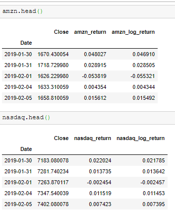
We will get the closing values for both Amazon and NASDAQ and we will get the daily returns, both as a percentage change and as log returns. We do that because some analysts prefer to work with log returns and some others with daily returns. For our example, we will work with the simple daily returns.

import pandas as pd
import numpy as np
import yfinance as yf
from sklearn.linear_model import LinearRegression
import matplotlib.pyplot as plt
%matplotlib inline 

# get the closing price of AMZN Stock
amzn = yf.download('AMZN', start='2019-01-30', end='2021-01-30', progress=False)['Close']
amzn = pd.DataFrame(amzn)
amzn['amzn_return'] = amzn['Close'].pct_change()
amzn['amzn_log_return'] = np.log(amzn['Close']) - np.log(amzn['Close'].shift(1))
amzn.dropna(inplace=True)


# get the closing price of NASDAQ Index
nasdaq = yf.download('^IXIC', start='2019-01-30', end='2021-01-30', progress=False)['Close']
nasdaq = pd.DataFrame(nasdaq)
nasdaq['nasdaq_return'] = nasdaq['Close'].pct_change()
nasdaq['nasdaq_log_return'] = np.log(nasdaq['Close']) - np.log(nasdaq['Close'].shift(1))
nasdaq.dropna(inplace=True)
 

Build the Market Beta Rolling Regression function

For the rolling regression, we will create a function, which will take as input the Stock returns (Y) , the Index (X) and the time window.

def market_beta(X,Y,N):
    """ 
    X = The independent variable which is the Market
    Y = The dependent variable which is the Stock
    N = The length of the Window
    
    It returns the alphas and the betas of
    the rolling regression
    """
    
    # all the observations
    obs = len(X)
    
    # initiate the betas with null values
    betas = np.full(obs, np.nan)
    
    # initiate the alphas with null values
    alphas = np.full(obs, np.nan)
    
    
    for i in range((obs-N)):
        regressor = LinearRegression()
        regressor.fit(X.to_numpy()[i : i + N+1].reshape(-1,1), Y.to_numpy()[i : i + N+1])
        
        betas[i+N]  = regressor.coef_[0]
        alphas[i+N]  = regressor.intercept_

    return(alphas, betas)
 
results = market_beta(amzn.amzn_return, nasdaq.nasdaq_return, 30)

results = pd.DataFrame(list(zip(*results)), columns = ['alpha', 'beta'])

results

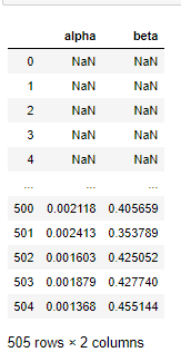
results.index = amzn.index
plt.figure(figsize=(12,8))
results.beta.plot.line()
plt.title("Market Beta: Amzn vs Nasdaq with Rolling Window of 30 Days")

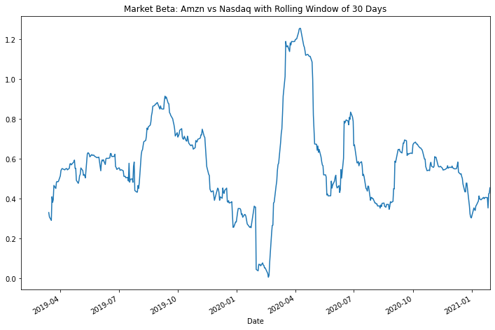
The Takeaway

As we can see, the market beta for Amazon versus Nasdaq lies mainly between 0 and 1. The rolling regression is a good approach to detect changes in the behavior of the stocks against the market. The approach of rolling regression can be applied in other things such as pairs trading and so on. It can also be applied to other assets like cryptocurrencies etc.