Example of Pairs Trading

Introduction

Statistical arbitrage trading is a quantitative and computational approach to equity trading that is widely applied by hedge funds to produce market-neutral returns. The simplest and most popular version of the strategy is known as pairs trading and involves the identification of pairs of assets that are believed to have some long-run equilibrium relationship. By taking an appropriate long-short position on this pair when the spread has diverged sufficiently from the equilibrium value, a profit will be made if the spread converges back to equilibrium by unwinding the position. Similar ideas govern more complicated strategies that consider a larger basket of assets. We will focus on pairs trading strategy endeavoring to
specify precisely the concept of the long-run equilibrium relationship between two stocks and then we try to describe and apply a computational methodology for modelling the mispricing dynamics. Before starting the analysis it is essential to clarify that statistical arbitrage
trading is not a riskless strategy and thus an investor who follows it should be alert.

Get the Stock Prices

We will work in R and we will get the stock prices using the quantmod package. For this example, we will take into consideration the closing prices of 30 arbitrary stocks from NASDAQ. Note that 30 stocks generate 435 pairs. In the real world, we use to work with thousands of stocks and millions of pairs. Let’s get the closing prices of the following 30 stocks from 2020-01-01 up to 2021-01-03:

• “GOOGL”
• “TSLA”
• “FB”
• “AMZN”
• “AAPL”
• “MSFT”
• “VOD”
• “ADBE”
• “NVDA”
• “CRM”
• “EBAY”
• “YNDX”
• “TRIP”
• “NFLX”
• “DBX”
• “ETSY”
• “PYPL”
• “EA”
• “BIDU”
• “TMUS”
• “SPLK”
• “CTXS”
• “OKTA”
• “MDB”
• “ZM”
• “INTC”
• “GT”
• “SBUX”
• “WIX”
• “ZNGA”

library(tidyverse)
library(tseries)
library(quantmod)

mySymbols <- c('GOOGL', 'TSLA', 'FB', 'AMZN', 'AAPL', 'MSFT', 'VOD',  'ADBE', 'NVDA', 'CRM',
               'EBAY', 'YNDX', 'TRIP', 'NFLX', 'DBX', 'ETSY', 'PYPL','EA', 'BIDU', 'TMUS',
               'SPLK', 'CTXS', 'OKTA', 'MDB', 'ZM', 'INTC', 'GT', 'SBUX', 'WIX', 'ZNGA')

myStocks <-lapply(mySymbols, function(x) {getSymbols(x, 
                                                             from = "2020-01-01", 
                                                             to = "2021-01-03",
                                                             periodicity = "daily",
                                                             auto.assign=FALSE)} )


names(myStocks)<-mySymbols


closePrices <- lapply(myStocks, Cl)
closePrices <- do.call(merge, closePrices)

names(closePrices)<-sub("\\.Close", "", names(closePrices))
head(closePrices)

Construct the Pairs

The aim of this strategy is to construct a portfolio of two stocks that are in long-run equilibrium. Then we take an appropriate position when the spread has diverged significantly from its equilibrium. A profit may be made by unwinding the position upon the convergence of the spread, or the measure of relative mispricing. From the above discussion, it is clear that we are seeking stocks whose price movements are strongly correlated in order to have chances to implement the pairs trading strategy. The simplest method to define potentially co-integrated pairs is the computation of the correlation of stock prices considering around 220 daily closing prices. A widely used method is the ‘distance method’ where the co-movement in a pair is measured by what is known as the distance or the sum of squared differences between the two normalized price series. Finally, a rational method is to consider the logarithm of the stock prices and then to compute the correlation of them.

Our approach will be:

1. Split the data into train and test datasets. As a train dataset, we consider the first 220 observations and as a test dataset the remaining last 32 observations.
2. We take the logarithm of the closing prices.
3. On the train dataset we run the linear regression of \(log(p_t^A)=β \times log(p_t^B) +ε_t\) where \(p_t^A\) and \(p_t^B\) are the daily closing prices of stocks A and B respectively. The coefficient β is the co-integration coefficient and the stochastic term \(ε_t\) is the spread. Notice that we chose to run the regression without an intercept coefficient. This is not necessary since both approaches are correct.
4. For every pair, we get the correlation coefficient, the β coefficient and the p-value from the augmented Dickey–Fuller test (ADF). We apply the ADF test in order to detect the co-integrated pairs.
5. The qualified pairs are those which have a correlation coefficient greater than 95% and a p-value less than 5%

Let’s do it in R:

# train
train<-log(closePrices[1:220])

# test
test<-log(closePrices[221:252])




# get the correlation of each pair

left_side<-NULL
right_side<-NULL
correlation<-NULL
beta<-NULL
pvalue<-NULL

for (i in 1:length(mySymbols)) {
  for (j in 1:length(mySymbols)) {
    
    if (i>j) {
      left_side<-c(left_side, mySymbols[i])
      right_side<-c(right_side, mySymbols[j])
      correlation<-c(correlation, cor(train[,mySymbols[i]], train[,mySymbols[j]]))
      
      # linear regression withoout intercept
      m<-lm(train[,mySymbols[i]]~train[,mySymbols[j]]-1)
      beta<-c(beta, as.numeric(coef(m)[1]))
      
      # get the mispricings of the spread
      sprd<-residuals(m)
      
      # adf test
      pvalue<-c(pvalue, adf.test(sprd, alternative="stationary", k=0)$p.value)
      
    }
  }
  
}

df<-data.frame(left_side, right_side, correlation, beta, pvalue)

mypairs<-df%>%filter(pvalue<=0.05, correlation>0.95)%>%arrange(-correlation)
mypairs
 

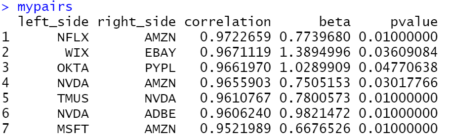
From the 435 pairs we kept the 7 pairs above.

Focus on a Pair

Let’s focus on the NFLX vs AMZN pair which consists of the Netflix and Amazon stocks respectively. Our strategy is when the spread diverges from 0 to open a position with the spread, hoping that it will converge again to its mean which is 0. Let’s plot the spread on the train dataset:

Train Dataset

myspread<-train[,"NFLX"]-0.7739680*train[,"AMZN"]
plot(myspread, main = "NFLX vs AMZN")
 

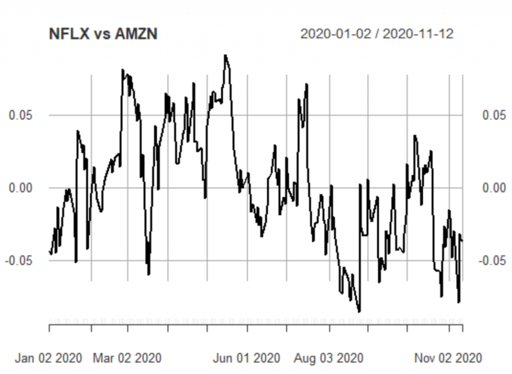
Analyzing the spread, we can define trading signals for when to open a position and when to close. We can use the quantiles or 3 standard deviations. For simplicity, let’s consider that our trading signals are 0.04 and -0.04 respectively. The strategy is the following:

• When the spread is above 0.04, then we sell the spread which means that we sell the NFLX and we buy AMZN
• When the spread is below -0.04, then we buy the spread which means that we buy NFLX and we sell AMZN
• Whenever the spread converges again to 0, then we close our position.

Test Dataset

Let’s have a look at the spread on the test dataset:

myspread<-test[,"NFLX"]-0.7739680*test[,"AMZN"]
plot(myspread, main = "NFLX vs AMZN")
 

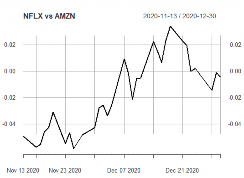
As we can see, on the 13th of November the spread was below -004 and as expected it converged to its mean on the 7th of December.

Conclusion

Pairs trading is a strategy that can be applied in both bearish and bullish markets. It is not a risk-free strategy since it is possible for one pair to never converge to its mean. Moreover, when we backtest the pairs trading strategies, we need to assume that the short selling is allowed and to take into consideration the transaction cost and the short-selling fees.

Get 25$ in BTC for FREE

You can get $25 in Bitcoin by investing $100 in Nexo