Skewness and Kurtosis in Statistics

Most commonly a distribution is described by its mean and variance which are the first and second moments respectively. Another less common measures are the skewness (third moment) and the kurtosis (fourth moment). Today, we will try to give a brief explanation of these measures and we will show how we can calculate them in R.

Skewness

The skewness is a measure of the asymmetry of the probability distribution assuming a unimodal distribution and is given by the third standardized moment.

We can say that the skewness indicates how much our underlying distribution deviates from the normal distribution since the normal distribution has skewness 0. Generally, we have three types of skewness.

• Symmetrical: When the skewness is close to 0 and the mean is almost the same as the median
• Negative skew: When the left tail of the histogram of the distribution is longer and the majority of the observations are concentrated on the right tail. In this case, we can use also the term “left-skewed” or “left-tailed”. and the median is greater than the mean.
• Positive skew: When the right tail of the histogram of the distribution is longer and the majority of the observations are concentrated on the left tail. In this case, we can use also the term “right-skewed” or “right-tailed”. and the median is less than the mean.

The graph below describes the three cases of skewness. Focus on the Mean and Median.

Skewness formula

The skewness can be calculated from the following formula:

\(skewness=\frac{\sum_{i=1}^{N}(x_i-\bar{x})^3}{(N-1)s^3}\)

where:

• σ is the standard deviation
• \( \bar{x }\) is the mean of the distribution
• N is the number of observations of the sample

Skewness values and interpretation

There are many different approaches to the interpretation of the skewness values. A rule of thumb states that:

• Symmetric: Values between -0.5 to 0.5
• Moderated Skewed data: Values between -1 and -0.5 or between 0.5 and 1
• Highly Skewed data: Values less than -1 or greater than 1

Skewness in Practice

Let’s calculate the skewness of three distribution. We will show three cases, such as a symmetrical one, and one positive and negative skew respectively.

We know that the normal distribution is symmetrical.

set.seed(5)

# normal
x = rnorm(1000, 0,1)
hist(x, main="Normal: Symmetrical", freq=FALSE)
lines(density(x), col='red', lwd=3)
abline(v = c(mean(x),median(x)),  col=c("green", "blue"), lty=c(2,2), lwd=c(3, 3))
 

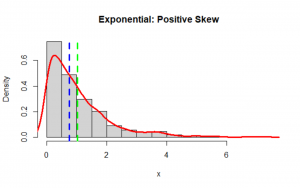
The exponential distribution is positive skew:

set.seed(5)
# exponential
x = rexp(1000,1)
hist(x, main="Exponential: Positive Skew", freq=FALSE)
lines(density(x), col='red', lwd=3)
abline(v = c(mean(x),median(x)),  col=c("green", "blue"), lty=c(2,2), lwd=c(3, 3))
  

The beta distribution with hyper-parameters α=5 and β=2

set.seed(5)
# beta
x= rbeta(10000,5,2)
hist(x, main="Beta: Negative Skew", freq=FALSE)
lines(density(x), col='red', lwd=3)
abline(v = c(mean(x),median(x)),  col=c("green", "blue"), lty=c(2,2), lwd=c(3, 3))
 

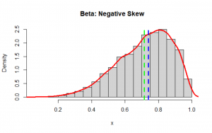
Notice that the green vertical line is the mean and the blue one is the median.

Let’s see how we can calculate the skewness by applying the formula:

set.seed(5)
x= rbeta(10000,5,2)

sum((x-mean(x))^3)/((length(x)-1)*sd(x)^3)
 

We get:

3.085474

Notice that you can also calculate the skewness with the following packages:

library(moments)
moments::skewness(x) 

# OR

library(e1071)
e1071::skewness(x) 

There are some rounding differences between those two packages. Also at the e1071 the formula is without subtracting the 1from the (N-1).

Kurtosis

In statistics, we use the kurtosis measure to describe the “tailedness” of the distribution as it describes the shape of it. It is also a measure of the “peakedness” of the distribution. A high kurtosis distribution has a sharper peak and longer fatter tails, while a low kurtosis distribution has a more rounded pean and shorter thinner tails.

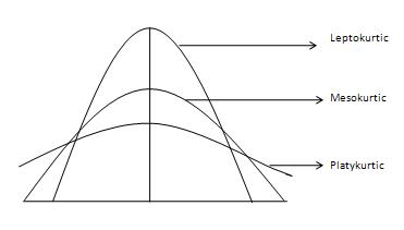
Let’s see the main three types of kurtosis.

• Mesokurtic: This is the normal distribution
• Leptokurtic: This distribution has fatter tails and a sharper peak. The kurtosis is “positive” with a value greater than 3
• Platykurtic: The distribution has a lower and wider peak and thinner tails. The kurtosis is “negative” with a value less than 3

Notice that we define the excess kurtosis as kurtosis minus 3

Kurtosis formula

The kurtosis can be derived from the following formula:

\(kurtosis=\frac{\sum_{i=1}^{N}(x_i-\bar{x})^4}{(N-1)s^4}\)

where:

• σ is the standard deviation
• \( \bar{x }\) is the mean of the distribution
• N is the number of observations of the sample

Kurtosis interpretation

Kurtosis is the average of the standardized data raised to the fourth power. Any standardized values that are less than 1 (i.e., data within one standard deviation of the mean, where the “peak” would be), contribute virtually nothing to kurtosis, since raising a number that is less than 1 to the fourth power makes it closer to zero. The only data values (observed or observable) that contribute to kurtosis in any meaningful way are those outside the region of the peak; i.e., the outliers. Therefore, kurtosis measures outliers only; it measures nothing about the “peak”.

Kurtosis in Practice

Let’s try to calculate the kurtosis of some cases:

Normal Distribution

set.seed(5)
# normal
x = rnorm(1000, 0,1)
sum((x-mean(x))^4)/((length(x)-1)*sd(x)^4)
 

[1] 3.058924

As expected we got a value close to 3!

Exponential distribution

set.seed(5)
# exponential
x = rexp(1000)
sum((x-mean(x))^4)/((length(x)-1)*sd(x)^4)
 

[1] 10.13425

As expected we get a positive excess kurtosis (i.e. greater than 3) since the distribution has a sharper peak.

Beta distribution

set.seed(5)
# beta
x = rbeta(1000,5,5)
sum((x-mean(x))^4)/((length(x)-1)*sd(x)^4)
 

[1] 2.634339

As expected we get a negative excess kurtosis (i.e. less than 3) since the distribution has a lower peak.

Notice that you can also calculate the kurtosis with the following packages:

library(moments)
moments::kurtosis(x) 

# OR 
# By default it caclulates the excess kurtosis so you have to add 3
library(e1071)
e1071::kurtosis(x, type=1)+3

---

Conclusion

We provided a brief explanation of two very important measures in statistics and we showed how we can calculate them in R. I would suggest that apart from sharing only the mean and the variance of the distribution to add also the skewness and the kurtosis since we get a better understanding of the data.