We will provide you an example of how you can start building your predictive sport model, specifically for soccer, but you can extend the logic to other sports as well. We will provide the steps that we need to follow:
Get the Historical Data Regularly
The first thing that we need to do is to get the historical data of the past games, including the most recent ones. The data should be updated regularly. This is a relatively challenging part. You can either try to get the data on your own by applying scraping or you can get the data through an API where usually there is a fee. Let’s assume that we have arranged how will get the historical data on a regular basis. Below, we provide an example of how the data usually look like:

As we can see are tabular data, let’s return the column names
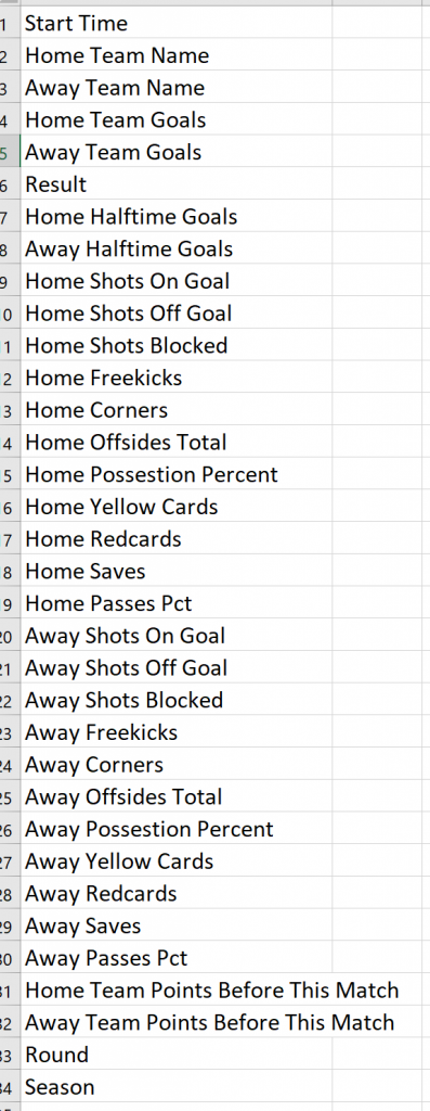
As we can see, this data referred to the outcome of each game. We will need to create other features for our predictive model.
Feature Engineering
The logic is that before each game, (example Southampton vs Chelsea) we would like to know the average features of each team up to that point. This implies that we need to work on the data in order to transform them in the proper form. So before each game, we want to know, how many goals does Southampton scores on average when it plays Home, how many received when it plays Away and the same for the opponent, which is Chelsea in our example. Clearly, this should be extended to all features.
We will need to group the data per Season and Team. We will need to create features when the teams play Away and when the play Home. So each team, no matter if the next game is Home or Away, will have values for both Home and Away features. Finally, we will need to join the “Home” team Data Frame with the “Away” team Data Frame based on the match that we want to predict or to train the model.
Let’s see how we can do this in R. Notice that we use the “lag” function because we can to get the data up until this game and NOT including the game since in theory, we do not know the outcome and we use also the “cummean” function which returns the cumulative mean
Home Features
library(tidyverse)

# Read the csv file of the data obtained from the API
df<-read.csv("premierleague20162020.csv", sep=";")


# Create the "Home" Data Frame

H_df<-df%>%select(-Start.Time, - Away.Team.Name,-Result)%>%
      group_by(Season, Home.Team.Name)%>%arrange(Round)%>%
      mutate_at(vars(Home.Team.Goals:Away.Passes.Pct), funs(lag))%>%
      na.omit()%>%
      mutate_at(vars(Home.Team.Goals:Away.Passes.Pct), funs(cummean))%>%
      select(-Away.Team.Points.Before.This.Match)%>%ungroup()


# Add a prefix of "H_" for all the home features:

colnames(H_df)<-paste("H", colnames(H_df), sep = "_")
Away Features
# Create the "Avay" Data Frame

A_df<-df%>%select(-Start.Time, - Home.Team.Name, -Result)%>%
      group_by(Season, Away.Team.Name)%>%arrange(Round)%>%
      mutate_at(vars(Home.Team.Goals:Away.Passes.Pct), funs(lag))%>%
      na.omit()%>%
      mutate_at(vars(Home.Team.Goals:Away.Passes.Pct), funs(cummean))%>%
      select(-Home.Team.Points.Before.This.Match)%>%ungroup()


# Add a prefix of "A_" for all the away features:

colnames(A_df)<-paste("A", colnames(A_df), sep = "_")
Results Data Frame
We keep also the results data frame which consists of the Round, Season, Home.Team.Name, Away.Team.Name and the Result of the game.
# keep the table with the actual results

results_df<-df%>%select(Round, Season, Home.Team.Name,   Away.Team.Name, Result)
Final Data Frame
The final data frame consists of the three data frames above. So, we will need to join them
# join the three data frames
final_df<-results_df%>%
          inner_join(H_df, by=c("Home.Team.Name"="H_Home.Team.Name", "Round"="H_Round", "Season"="H_Season"))%>%
          inner_join(A_df, by=c("Away.Team.Name"="A_Away.Team.Name", "Round"="A_Round", "Season"="A_Season"))
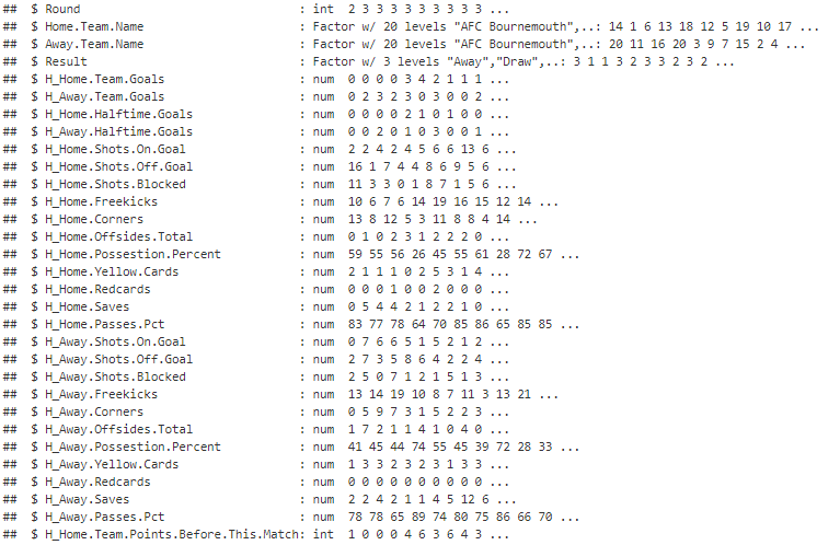
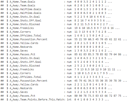
The final features for this dataset will be the Season plus the :
Build the Machine Learning Model
Now we are ready to build the machine learning model. We can adjust the dependent variable that we want to predict based on our needs. It can be the “Under/Over“, the “Total Number of Goals” the “Win-Loss-Draw” etc. In our case, the “y” variable is the result that takes 3 values such as “Win”, “Loss” and “Draw”. I.e. for R this is a factor of 3 levels. Let’s see how we can build a classification algorithm working with R and H2O.
library(h2o)
h2o.init()

Train<-final_df%>%filter(Round<=29, Round>=6)
Test<-final_df%>%filter(Round>=30)

Train_h2o<-as.h2o(Train)
Test_h2o<-as.h2o(Test)

# auto machine learning model. Will pick the best one
aml <- h2o.automl(y = 5,  x=6:62, training_frame = Train_h2o,   leaderboard_frame  = Test_h2o, max_runtime_secs = 60)

# pick the best model
lb <- aml@leaderboard


# The leader model is stored here
# aml@leader
#pred <- h2o.predict(aml, test)
# or
#pred <- h2o.predict(aml@leader, Test_h2o)


h2o.performance(model = aml@leader, newdata = Train_h2o)
Clearly, for betting purposes, we do not care so much about the predictive outcome of the model but mostly about the odds of each outcome so that to take advantage of bookies mispricing.
Discussion
The model that we described above is a reliable starting model. We can improve it by enriching it with other features like players’ injuries, team budget, other games within a week (eg Champions League Games) etc. However, always the logic remains the dame, we have the “X” features which are up until the most recent game and our “y” which is what we want to predict. There are also other techniques where we can give more weight to the most recent observations. Generally speaking, there is much research on predictive soccer games.

