Linear Regression
Linear regression is a basic approach to modelling the linear relationship between a dependent variable y and one or more independent variables X. The equation of the linear regression is:

for each observation i=1,2,…,n.
When we run a linear regression model, we conduct hypothesis testing on the regression coefficients. The null hypothesis is that the beta coefficient is 0 versus the alternative hypothesis that is not zero.
\(H_0:\beta_i=0\)
\(H_1:\beta_i\neq0\)
When we reject the null hypothesis it implies that the coefficient βi of the corresponding variable Xi is not zero and as a result is statistically significant. The significance level α usually takes values 0.01, 0.05, and 0.10. The lower the value the stricter to reject the null hypothesis.
Type I Error
In hypothesis testing we have two types of error, such as the:
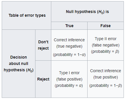
- Type I Error: It is the rejection of the null hypothesis when the null hypothesis is true. It is also known as “false positive”. For example, consider an innocent person that is convicted.
- Type II Error: It is the non-rejection of the null hypothesis when the null hypothesis is false. It is also known as “false negative”. For example, consider a guilty person that is not convicted.
The table below represents the error types.

Today, we will focus on Type I error. In statistics, we are aware of the significance level α, which is the probability to reject the null hypothesis, given that the null hypothesis was assumed to be true and the p-value is the probability of obtaining a result at least as extreme, given that the null hypothesis is true. In other words, the level of significance α is the probability of making a type I error. In most cases, α=5% implies that we are willing to accept a 5% chance to mistakenly reject the null hypothesis.
Example of Linear Regression and Type I Error
Let’s assume that I generate 100 random variables from the standard normal distribution (Xs) and I run a Multivariate Linear Regression on another standard normal variable (y). The question is how many statistically significant variables do you expect to get at a 5% level of confidence?
Someone could argue that since the 100 independent variables are randomly generated, then none should be statistically significant. But as we said before, we expect to reject the null hypothesis (i.e. to claim that the variable is statistically significant) where the null hypothesis is true. Thus, if we reject the null hypothesis at 5% level of confidence α, then we expect to see 5 out of 100 random variables to appear to be statistically significant. In order to prove this scenario we will run a simulation:
- Generate 100 independent variables from the standard normal of 1000 observations each. These are the 100 independent variables X
- Generate 1000 observations from the standard normal. This is the dependent variable y.
- Run a multivariate linear regression on y with all the independent variables X.
- Count how many variables found to be statistically significant at 5% level of significance. (p-value less than 5%)
- Repeat this analysis 1000 times and report the distribution of the number of significant variables.
significant_variables<-c()


for (i in 1:1000) {
      df = data.frame(matrix(rnorm(101*1000,0,1), nrow=1000))

      model<-lm(X101~., data=df)


      output<-summary(model)$coefficients

      # remove the intercept from the output
      output<-output[rownames(output)!="(Intercept)",]

      tmp<-dim(output[output[,4]<0.05,])[1]

      significant_variables<-c(significant_variables, tmp)
     }

hist(significant_variables, main="Number of Significant Variables")

Let’s get also the summary of the number fo significant variables.
> summary(significant_variables)
   Min. 1st Qu.  Median    Mean 3rd Qu.    Max.
  0.000   3.000   5.000   5.112   6.000  16.000
As we can see the mean is 5.112 and the median is 5. This is a very nice example to understand the Type I Error.
Discussion
We explained in action how we can get false statistically significant variables. We need to keep this in mind when we report which variables are actually statistically significant and to stress out the probability of Type I Error. This phenomenon is more common when we are dealing with multiple comparisons. We have provided some examples of multiple comparisons such as the ANOVA vs Multiple Comparisons and AB Testing


