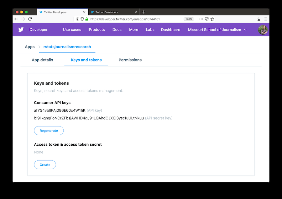
In a previous post, we showed how to get Twitter data using Python. In this tutorial, we will show you how to get Twitter data using R and more particularly with the rtweet library. As we have explained in the previous post, you will need to create a developer account and get your consumer and access keys respectively.
Install the rtweet Library and API Authorization
We can install the rtweet library either from CRAN or from GitHub as follows:
## install rtweet from CRAN
install.packages("rtweet")


## OR
## install remotes package if it's not already
if (!requireNamespace("remotes", quietly = TRUE)) {
  install.packages("remotes")
}

## install dev version of rtweet from github
remotes::install_github("ropensci/rtweet")
Then we are ready to load the library:
## load rtweet package
library(rtweet)
We can authorize the API by entering our credentials:

## load rtweet
library(rtweet)

## load the tidyverse
library(tidyverse)

## store api keys (these are fake example values; replace with your own keys)
api_key <- "afYS4vbIlPAj096E60c4W1fiK"
api_secret_key <- "bI91kqnqFoNCrZFbsjAWHD4gJ91LQAhdCJXCj3yscfuULtNkuu"

## authenticate via web browser
token <- create_token(
  app = "rstatsjournalismresearch",
  consumer_key = api_key,
  consumer_secret = api_secret_key)

get_token()
Search Tweets
Now we are ready to get our first data from Twitter, starting with 1000 tweets containing the hashtag “#DataScience” by excluding the re-tweets. Note that the “search_tweets” returns data from the last 6-9 days
rt <- search_tweets("#DataScience", n = 1000, include_rts = FALSE)
View(rt)
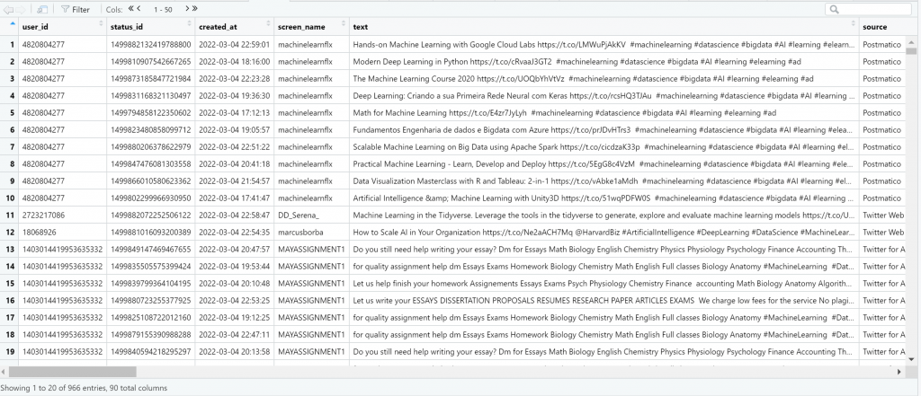
Usually, we want to get the screen name, the text, the number of likes and the number of re-tweets.
View(rt%>%select(screen_name, text, favorite_count, retweet_count))
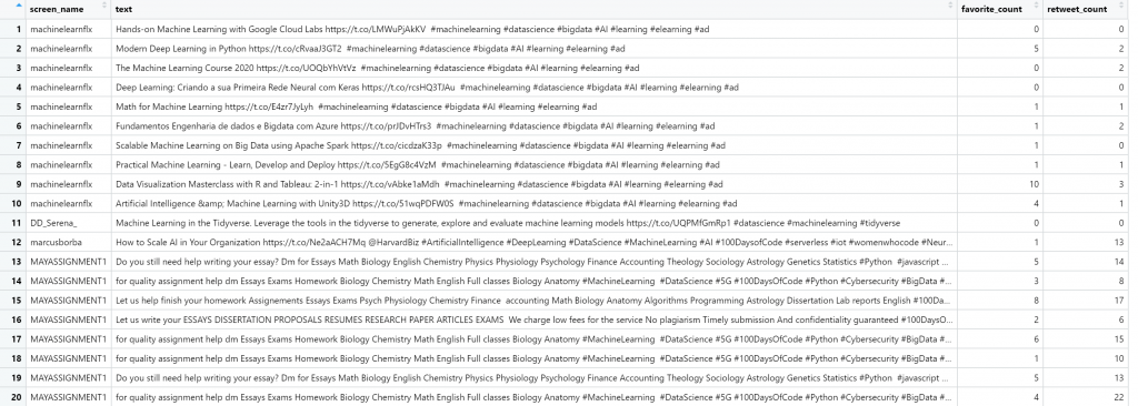
The rt object consists of 90 columns, so as you can understand it contains a lot of information. Note that there is a limit of 18000 tweets per 15 minutes. If we want to get more, we should do the following:
## search for 250,000 tweets containing the word datascience
rt <- search_tweets(
  "datascience", n = 250000, retryonratelimit = TRUE
)
We can also plot the tweets:
ts_plot(rt, "hour")

Stream Tweets
Stream tweets return a random sample of approximately 1% of the live stream of all tweets, having the option to filter the data via a search-like query, or enter specific user ids, or define the geo-coordinates of the tweets.
## stream tweets containing the toke DataScience for 30 seconds
rt <- stream_tweets("DataScience", timeout = 30)
View(rt)
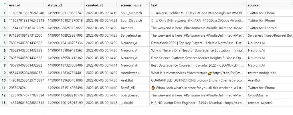
Note that the rt object consists of 90 columns.
Filter Tweets
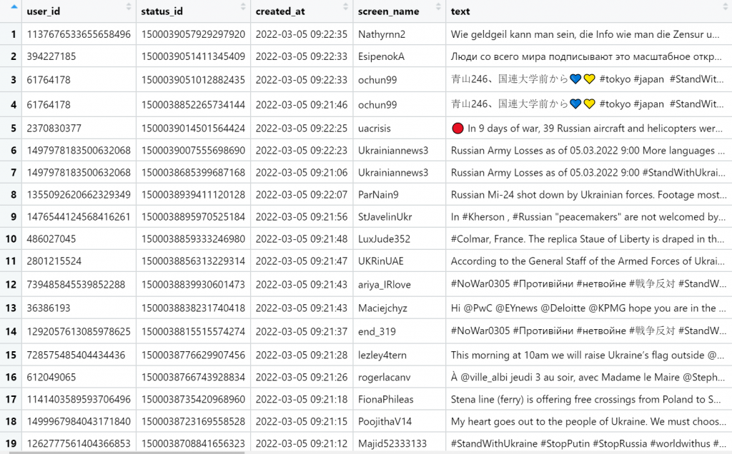
When we search for tweets, we can also apply some filters. For example, let’s say that we want to specify the language or to exclude retweets and so on. Let’s search for tweets that contain the “StandWithUkraine” text by excluding retweets, quotes and replies.
ukraine <- search_tweets("StandWithUkraine-filter:retweets -filter:quote -filter:replies", n = 100)
View(ukraine)
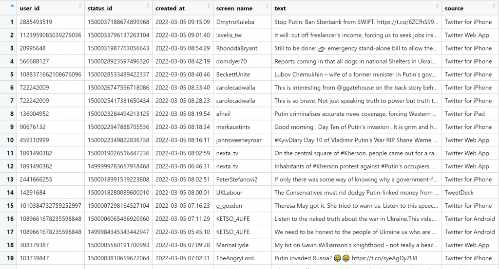
Finally, let’s search for tweets in English that contain the word “Putin” and have more than 100 likes and retweets.
putin<-search_tweets("Putin min_retweets:100 AND min_faves:100", lang='en')
View(putin)
Get Timelines
The get_imeline() function returns up to 3,200 statuses posted to the timelines of each of one or more specified Twitter users. Let’s get the timeline of R-bloggers and Hadley Wickham accounts by taking into consideration the 500 most recent tweets of each one.
rt<-get_timeline(user=c("Rbloggers", "hadleywickham"), n=500)
Whose tweets are more popular? Who gets more likes and retweets? Let’s answer this question.
rt%>%group_by(screen_name)%>%
     summarise(AvgLikes = mean(favorite_count, na.rm=TRUE), AvgRetweets = mean(retweet_count, na.rm=TRUE))
As we can see, the guru Hadley Wickham gets much more likes and retweets compared to R-bloggers.
# A tibble: 2 x 3
  screen_name   AvgLikes AvgRetweets
1 hadleywickham     31.6     110.
2 Rbloggers         17.8     6.17
Get the Likes made by a User
We can get the n most recently liked tweets by a user. Let’s see what Hadley likes!
hadley <- get_favorites("hadleywickham", n = 1000)
Which are his favorite accounts?
hadley%>%group_by(screen_name)%>%count()%>%arrange(desc(n))%>%head(5)
And we get:
# A tibble: 5 x 2
# Groups:   screen_name [5]
  screen_name       n
1 djnavarro        17
2 ijeamaka_a       13
3 mjskay           12
4 sharlagelfand    12
5 vboykis          12
Which are his favorite hashtags?
hadley%>%unnest(hashtags)%>%group_by(tolower(hashtags))%>%count()%>%
      arrange(desc(n))%>%na.omit()%>%head(5)
And we get:
# A tibble: 5 x 2
# Groups:   tolower(hashtags) [5]
  `tolower(hashtags)`     n
1 rstats                 78
2 rtistry                22
3 genuary2022             9
4 genuary                 7
5 rayrender               6
Search Users
We can search for users with a specific hashtag. For example:
## search for up to 1000 users using the keyword rstats
rstats <- search_users(q = "rstats", n = 1000)

## data frame where each observation (row) is a different user
rstats

## tweets data also retrieved. can access it via tweets_data()
tweets_data(rstats)
Get Friends and Followers
We can get the user ids of the friends and followers of a specific account. Let’s get the friends and followers of the Predictive Hacks account.
get_followers("predictivehacks")
get_friends("predictivehacks")
We can extract more info on the user ids using the function:
lookup_users(users, parse = TRUE, token = NULL)
where users is a user id or screen name of the target user.
Get Trends
We can get the trends in a particular city or country. For example:
## Retrieve available trends
trends <- trends_available()
trends

## Store WOEID for Worldwide trends
worldwide <- trends$woeid[grep("world", trends$name, ignore.case = TRUE)[1]]

## Retrieve worldwide trends datadata
ww_trends <- get_trends(worldwide)

## Preview trends data
ww_trends

## Retrieve trends data using latitude, longitude near New York City
nyc_trends <- get_trends_closest(lat = 40.7, lng = -74.0)

## should be same result if lat/long supplied as first argument
nyc_trends <- get_trends_closest(c(40.7, -74.0))

## Preview trends data
nyc_trends

## Provide a city or location name using a regular expression string to
## have the function internals do the WOEID lookup/matching for you
(luk <- get_trends("london"))
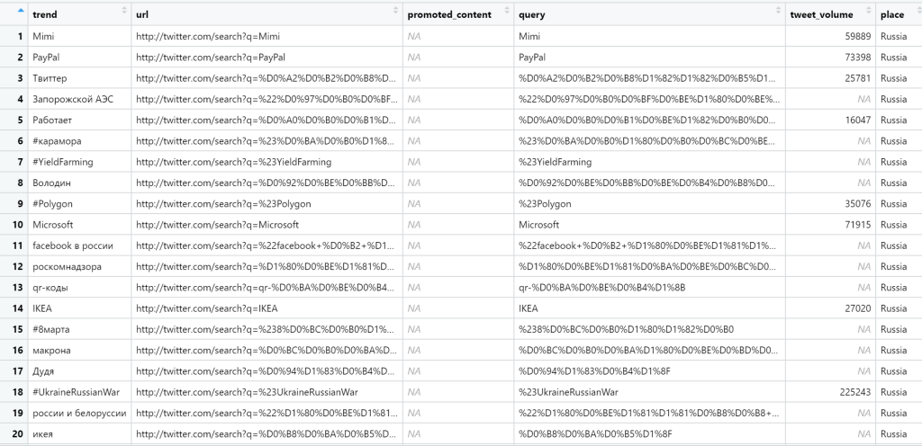
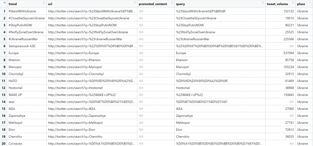
Let’s see what is trending in Russia and in Ukraine, respectively.
get_trends("Russia")
get_trends("Ukraine")
Final Thoughts
Every Data Science analysis starts with the data. In this tutorial, we showed how to get Twitter data in R. In the next posts, we will show you how to analyze this data by applying sentiment analysis, topic modelling, network analysis and so on. Stay tuned!


