
This is a quick tutorial about Social Network Analysis using Networkx taking as examples the characters of Game of Thrones. We got the data from the github merging all the 5 books and ignoring the “weight” attribute.
Social Network Analysis
With Network Science we can approach many problems. Almost everything could be translated to a “Network” with Nodes and Edges. For example, the Google Maps is a network where the Nodes could be the “Places” and Edges can be the “Streets”. Of course the most famous network is the Facebook which is an “undirected” graph and the Instagram which is “directed” since we have the people that we follow and our followers. The nodes are the “users” and the “edges” are the connections between them. Notice that both “nodes” and “edges” can have attributes. For example, node attributes in Facebook can be the “Gender”, “Location”, “Age” etc and edge attribute can be “date of last conversation between two nodes”, ‘number of likes”, “date they connected” etc.
Notice that with Network Analysis we can apply recommendation systems but this is out of the scope of this tutorial.
Game of Thrones in NetworkX
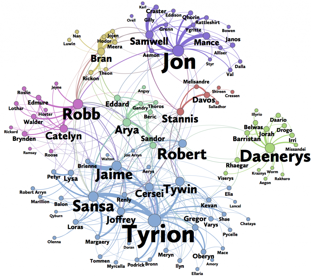
We will use the NetworkX python library on “Game of Thrones” data. The first exercise is to load the data and to get the number of nodes of the network which is 796 and the number of edges which is 2823. Thus, we are dealing with 796 characters of Game of Thrones.
import networkx as nx
import nxviz as nv
import pandas as pd
import matplotlib.pyplot as plt
%matplotlib inline

# read all the 5 csv files
# keep only the distinct pairs of source target since we will ignore the books and the weights

all_books = ["book1.csv", "book2.csv", "book3.csv", "book4.csv", "book5.csv"]

li = []

for f in all_books:
    tmp = pd.read_csv(f)
    li.append(tmp)

df = pd.concat(li, axis=0, ignore_index=True)

df = df[['Source', 'Target']]
df.drop_duplicates(subset=['Source', 'Target'], inplace=True)


# create the networkx object

G = nx.from_pandas_edgelist(df,  source='Source', target='Target')

# How to get the number of nodes

print(len(G.nodes()))

# How to get the number of edges

print(len(G.edges()))
We will return some of the main Network properties such as “average shortest path length“, “diameter“, “density“, “average clustering” and “transitivity“. We commend out the answers of each property.
As we will see the “diameter” of our graph is 9, which is the longest of all the calculated shortest paths in a network. It is the shortest distance between the two most distant nodes in the network. In other words, once the shortest path length from every node to all other nodes is calculated, the diameter is the longest of all the calculated path lengths. The diameter is representative of the linear size of a network.
Also the “average shortest path length” is 3.41 which is calculated by finding the shortest path between all pairs of nodes, and taking the average over all paths of the length thereof. This shows us, on average, the number of steps it takes to get from one member of the network to another
nx.average_shortest_path_length(G)
# 3.416225783003066

nx.diameter(G)
# 9

nx.density(G)
# 0.008921968332227173

nx.average_clustering(G)
# 0.4858622073350485

nx.transitivity(G)
# 0.2090366938564282
Centrality Measures
We are going to represent some Centrality measures. We give the definition of the most common:
- Degree centrality of a node in a network is the number of links (vertices) incident on the node.
- Closeness centrality determines how “close” a node is to other nodes in a network by measuring the sum of the shortest distances (geodesic paths) between that node and all other nodes in the network.
- Betweenness centrality determines the relative importance of a node by measuring the amount of traffic flowing through that node to other nodes in the network. This is done by measuring the fraction of paths connecting all pairs of nodes and containing the node of interest. Group Betweenness centrality measures the amount of traffic flowing through a group of nodes.
We will return also the famous PageRank although it is most common in “directed” graphs.
Based on this centrality measures, we will define the 5 more important characters in Game of Thrones.
# Compute the betweenness centrality of G: bet_cen
bet_cen = nx.betweenness_centrality(G)
# Compute the degree centrality of G: deg_cen
deg_cen = nx.degree_centrality(G)
# Compute the page rank of G: page_rank
page_rank = nx.pagerank(G)
# Compute the closeness centrality of G: clos_cen
clos_cen = nx.closeness_centrality(G)
sorted(bet_cen.items(), key=lambda x:x[1], reverse=True)[0:5]
[('Jon-Snow', 0.19211961968354493),
 ('Tyrion-Lannister', 0.16219109611159815),
 ('Daenerys-Targaryen', 0.11841801916269228),
 ('Theon-Greyjoy', 0.11128331813470259),
 ('Stannis-Baratheon', 0.11013955266679568)]
sorted(deg_cen.items(), key=lambda x:x[1], reverse=True)[0:5]
[('Tyrion-Lannister', 0.15345911949685534),
 ('Jon-Snow', 0.14339622641509434),
 ('Jaime-Lannister', 0.1270440251572327),
 ('Cersei-Lannister', 0.1220125786163522),
 ('Stannis-Baratheon', 0.11194968553459118)]
sorted(page_rank.items(), key=lambda x:x[1], reverse=True)[0:5]
[('Jon-Snow', 0.01899956924856684),
 ('Tyrion-Lannister', 0.018341232619311032),
 ('Jaime-Lannister', 0.015437447356269757),
 ('Stannis-Baratheon', 0.013648810781186758),
 ('Arya-Stark', 0.013432050115231265)]
sorted(clos_cen.items(), key=lambda x:x[1], reverse=True)[0:5]
[('Tyrion-Lannister', 0.4763331336129419),
 ('Robert-Baratheon', 0.4592720970537262),
 ('Eddard-Stark', 0.455848623853211),
 ('Cersei-Lannister', 0.45454545454545453),
 ('Jaime-Lannister', 0.4519613416714042)]
As we can see, for different Centrality measures, we get different results, for instance, “Jon-Snow” has the highest ” Betweenness” and “Tyrion-Lannister” the highest “Closeness” centrality.
Cliques
We will represent how we can get all the Cliques using NetworkX and we will show the largest one.
# get all cliques
all = nx.find_cliques(G)

# get the largest clique
largest_clique = sorted(nx.find_cliques(G), key=lambda x:len(x))[-1]

largest_clique
['Tyrion-Lannister',
 'Cersei-Lannister',
 'Joffrey-Baratheon',
 'Sansa-Stark',
 'Jaime-Lannister',
 'Robert-Baratheon',
 'Eddard-Stark',
 'Petyr-Baelish',
 'Renly-Baratheon',
 'Varys',
 'Stannis-Baratheon',
 'Tywin-Lannister',
 'Catelyn-Stark',
 'Robb-Stark']
Recommendations
You noticed that Facebook suggests you friends. There are many algorithms, but one of these is based on the “Open Triangles” which is a concept in social network theory. Triadic closure is the property among three nodes A, B, and C, such that if a strong tie exists between A-B and A-C, there is a weak or strong tie between B-C. This property is too extreme to hold true across very large, complex networks, but it is a useful simplification of reality that can be used to understand and predict networks.
Let’s try to make the top ten suggestions based on the “Open Triangles”
# Import necessary modules
from itertools import combinations
from collections import defaultdict

# Initialize the defaultdict: recommended
recommended = defaultdict(int)

# Iterate over all the nodes in G
for n, d in G.nodes(data = True):

    # Iterate over all possible triangle relationship combinations
    for n1, n2 in combinations(G.neighbors(n), 2):

        # Check whether n1 and n2 do not have an edge
        if not G.has_edge(n1, n2):

            # Increment recommended
            recommended[(n1, n2)] += 1

# Identify the top 10 pairs of users
all_counts = sorted(recommended.values())
top10_pairs = [pair for pair, count in recommended.items() if count > all_counts[-10]]
print(top10_pairs)
[('Catelyn-Stark', 'Tommen-Baratheon'), ('Eddard-Stark', 'Brienne-of-Tarth'), ('Petyr-Baelish', 'Brienne-of-Tarth'), ('Rodrik-Cassel', 'Stannis-Baratheon'), ('Arya-Stark', 'Brienne-of-Tarth'), ('Arya-Stark', 'Stannis-Baratheon'), ('Bran-Stark', 'Jaime-Lannister'), ('Bran-Stark', 'Stannis-Baratheon')]So for example we suggest connecting ‘Catelyn-Stark’ with ‘Tommen-Baratheon’ etc!