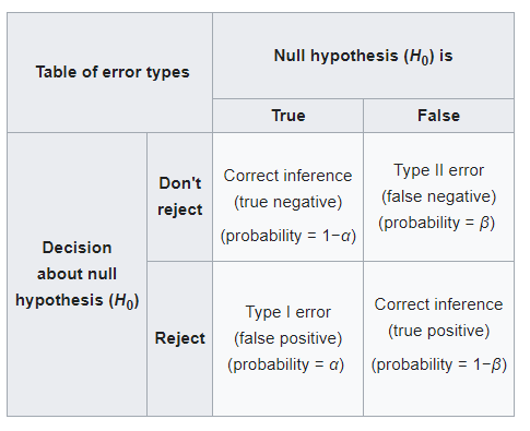
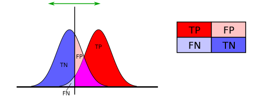
In this tutorial we will show how you can get the Power of Test when you apply Hypothesis Testing with Binomial Distribution. Before we provide the example let’s recall that is the Type I, and Type II errors.
Type I error
This is the probability to reject the null hypothesis, given that the null hypothesis is true. This is the level of significance α and in statistics is usually set to 5%
Type II error
This is the probability to accept the null hypothesis, given that the null hypothesis is false. In statistics, the Type II error is the β and is usually around 20%.
Power of Test
This is the probability to reject the null hypothesis, given that the null hypothesis is false. In statistics, we call it Power of γ and it is equal to 1-β and usually it takes values around 80%.
The table below summaries what we said above:

Power of a test
the power indicates the probability of avoiding a type II error and can be written as:
\(Power = P_r(H_1 | H_1)\)
Power analysis can be used to calculate the minimum sample size required to detect a statistical significance in Hypothesis Testing. The factors which affect the power are:
- The level of significance α, known as Type I Error.
- The difference of the observed and the theoretical value of the population in hypothesis testing.
- The sample size.
Power of Test: One-Sided Hypothesis Testing of Binomial Distribution
Problem: We took a sample of 24 people and we found that 13 of them are smokers. Can we claim that the proportion of smokers in the population is at least 35% at a 5% level of significance? What is the Power of Test?
Solution:
The problem can be formulated as follows:
\(H_0: p \leq 0.35\)
\(H_1: p \geq 0.35\)
The first thing that we should do is to find the critical value. We reject the null hypothesis for every value which is equal to or greater than the critical value. We can find it in different ways. Let’s get find the critical value with a for loop using the binom.test function.
x<-13
n<-24
p_test<-0.35
alpha<-0.05

critical<-NULL
for (i in c(0:n)) {

  if (binom.test(i, n, p=p_test, "greater")$p.value<alpha) {
    critical<-i
    break
  }

}
critical
Output:
[1] 13
Alternatively, we could have solved by calculating the quantile function which is the inverse CDF it as follows:
qbinom(0.95, 24, 0.35)
Output:
[1] 12
But we want the critical value to be greater than the value of the inverse CDF due to the discreteness of binomial distribution. So the critical value is 13. We can confirm it by summing up the probabilities using the PDF as follows:
sum(dbinom(13:24, 24, 0.35))
Output:
[1] 0.04225307
Note that the sum(dbinom(12:24, 24, 0.35)) is 0.09422976 greater than 0.05.
Calculate the Power of Test
Since we have found the critical value which is 13, let’s try to calculate the Power of Test γ. So we want to calculate the probability:
\(Power = P_r(X \geq c | n=24, p=13/24)= 1- P_r(X \geq (c-1) | n=24, p=13/24) = 1- P_r(X \leq12 | n=24, p=13/24)\)
Where \(X\) follows the binomial distribution, \(c\) is the critical value and \(p=13/24\) is the observed probability. We can easily calculate the power of test in R as follows:
1 - pbinom(critical-1, n, x/n)
Output:
[1] 0.5830354
Hence, the Power of Test is 58.30%
Power of Test: Two-Sided Hypothesis Testing of Binomial Distribution
Problem: We took a sample of 24 people and we found that 13 of them are smokers. Can we claim that the proportion of smokers in the population is 35% at a 5% level of significance? What is the Power of Test?
Solution:
The problem can be formulated as follows:
\(H_0: p = 0.35\)
\(H_1: p \neq 0.35\)
The first thing that we should do is to find the critical value. Since the test is two sided, we need to find two critical values. The critacal_minus and the critical_plus. Again we can work with the binom.test function. We will do two one-sided tests. A “greater” and a “less” as follows:
Note that the α is 0.05/2 since we are doing a two-sided test.
# two sided

x<-13
n<-24
p_test<-0.35
alpha<-0.05

critical_plus<-NULL
for (i in c(0:n)) {

  if (binom.test(i, n, p=p_test, "greater")$p.value<alpha/2) {
    critical_plus<-i
    break
  }

}
critical_plus


critical_minus<-NULL
for (i in c(n:0)) {

  if (binom.test(i, n, p=p_test, "less")$p.value<alpha/2) {
    critical_minus<-i
    break
  }

}
critical_minus
And we get as critical_minus and critical_plus the values 3 and 14 respectively. Alternatively, we could have used the inverse PDF as follows:
# critical minus
qbinom(0.025, 24, 0.35)-1
[1] 3

# critical plus
qbinom(0.975, 24, 0.35)+1
[1] 14
You can confirm that the critical values are correct since the probability beyond the critical values does not exceed the 0.05:
sum(dbinom(0:critical_minus, n, p_test))+sum(dbinom(critical_plus:n, n, p_test))
[1] 0.02968141
Calculate the Power of Test
Now we are ready to calculate the Power of Test. We will calculate it for both critical values and then we will add up the probabilities.
Critical Minus
\(Power = P_r(X \leq c_{minus} | n=24, p=13/24) = P_r(X \leq3 | n=24, p=13/24)\). Using R we get:
power_minus<-pbinom(critical_minus, n, x/n)
power_minus
[1] 2.773643e-05
Critical Plus
\(Power = P_r(X \geq c_{plus} | n=24, p=13/24)= 1- P_r(X \geq (c_{plus}-1) | n=24, p=13/24) = 1- P_r(X \leq13 | n=24, p=13/24)\). Using R we get:
power_plus<-1-pbinom(critical_plus-1, n, x/n)
power_plus
[1] 0.4213083
Power of the Test
Now, by adding the power_minus and the power_plus we get the power of the two-sided test with binomial distribution which is 42.13%:
power_minus+power_plus
[1] 0.421336


1 thought on “How to Get the Power of Test in Hypothesis Testing with Binomial Distribution”
I wonder, if there is an error the equation that determines the test power of the last example: 1 – Pr(X ≤ (cplus-1)|n=24, p=13/24). Since the probability of the counter event is calculated, the relation symbol should inverted.