
ARIMA is one of the most popular statistical models. It stands for AutoRegressive Integrated Moving Average and it’s fitted to time series data either for forecasting or to better understand the data. We will not cover the whole theory behind the ARIMA model but we will show you what’s the steps you need to follow to apply it correctly.
The key aspects of ARIMA model are the following:
- AR: Autoregression. This indicates that the time series is regressed on its own lagged values.
- I: Integrated. This indicates that the data values have been replaced with the difference between their values and the previous values in order to convert the series into stationary.
- MA: Moving Average. This indicates that the regression error is actually a linear combination of error terms whose values occurred contemporaneously and at various times in the past.
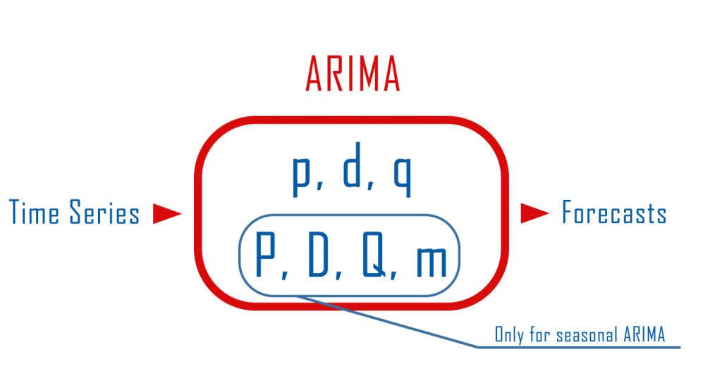
The ARIMA model can be applied when we have seasonal or non-seasonal data. The difference is that when we have seasonal data we need to add some more parameters to the model.
For non-seasonal data the parameters are:
- p: The number of lag observations the model will use
- d: The number of times that the raw observations are differenced till stationarity.
- q: The size of the moving average window.
For seasonal data we need to add also the following:
- P: The number of seasonal lag observations the model will use
- D: The number of times that the seasonal observations are differenced till stationarity.
- Q: The size of the seasonal moving average window.
- m: The number of observations of 1 season
Seasonal or Non-Seasonal Data
This is very easy to understand. Seasonal data is when we have intervals, such as weekly, monthly, or quarterly. For example, in this tutorial, we will use data that are aggregated by month and our “season” is the year. So, we have seasonal data and for the m parameter in the ARIMA model, we will use 12 which is the number of months per year.
Stationarity
ARIMA models can be applied only in stationary data. That means that we don’t want to have a trend in time. If the time series has a trend, then it’s non-stationary and we need to apply differencing to transform it into stationary. Below is an example of a stationary and a non-stationary series.

We can use also the Augmented Dickey-Fuller test to help us conclude if the series is stationary or not. The null hypothesis of the test is that there is a unit root with the alternative that there is no unit root. In other words, If the p-value is below 0.05 (or any critical size you will use), our Series is Stationary.
Let’s start coding.
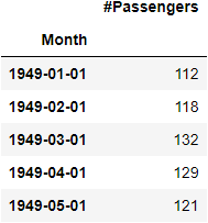
For this tutorial we will use the Air Passengers data from Kaggle.
import pandas as pd
import numpy as np
from statsmodels.tsa.seasonal import seasonal_decompose

#https://www.kaggle.com/rakannimer/air-passengers
df=pd.read_csv('AirPassengers.csv')

#We need to set the Month column as index and convert it into datetime
df.set_index('Month',inplace=True)
df.index=pd.to_datetime(df.index)

df.head()
First things first, let’s plot our data.
df.plot()
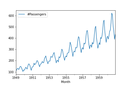
As you can clearly see, there is a trend in time and that suggests that the data are not stationary. However just to be sure we will use an Augmented Dickey-Fuller test.
from statsmodels.tsa.stattools import adfuller

result=adfuller(df['#Passengers'])

#to help you, we added the names of every value
dict(zip(['adf', 'pvalue', 'usedlag', 'nobs', 'critical' 'values', 'icbest'],result))
{'adf': 0.8153688792060468,
 'pvalue': 0.991880243437641,
 'usedlag': 13,
 'nobs': 130,
 'criticalvalues': {'1%': -3.4816817173418295,
  '5%': -2.8840418343195267,
  '10%': -2.578770059171598},
 'icbest': 996.692930839019}
As expected we failed to reject the Null Hypothesis and the series has a unit root thus is not stationary.
Transform Non-Stationary to Stationary using Differencing (the d and D parameters)
The next step is to transform our data to Stationary so we will have an estimate for d and D parameters we will use in the model. This can be done using Differencing and it’s performed by subtracting the previous observation from the current observation.
difference(T) = observation(T) – observation(T-1)
Then, we will test it again for stationarity using the Augmented Dickey-Fuller test and if it’s stationary we will proceed to our next step. If not we will apply differencing again till we have a stationary series. Differencing can be done very easily with pandas using the shift function.
df['1difference']=df['#Passengers']-df['#Passengers'].shift(1)

df['1difference'].plot()
It seems that we removed the trend and the series is Stationary. However we will use the Augmented Dickey-Fuller test to proove it.
#note we are dropping na values because the first value of the first difference is NA

result=adfuller(df['1difference'].dropna())
dict(zip(['adf', 'pvalue', 'usedlag', 'nobs', 'critical' 'values', 'icbest'],result))
{'adf': -2.8292668241699857,
 'pvalue': 0.05421329028382734,
 'usedlag': 12,
 'nobs': 130,
 'criticalvalues': {'1%': -3.4816817173418295,
  '5%': -2.8840418343195267,
  '10%': -2.578770059171598},
 'icbest': 988.5069317854084}
As you can see we fail to reject the null hypothesis because we have a p-value>0.05. That suggests that the series is not stationary and we need to use differencing again taking the second difference. The second difference can be computed as the first but this time instead of using the observations, we will use the first difference.
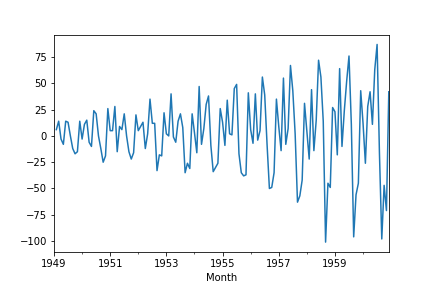
df['2difference']=df['1difference']-df['1difference'].shift(1)

df['2difference'].plot()

Let’s get the results from Augmented Dickey-Fuller test for the second difference.
result=adfuller((df['2difference']).dropna())
dict(zip(['adf', 'pvalue', 'usedlag', 'nobs', 'critical' 'values', 'icbest'],result))
{'adf': -16.384231542468452,
 'pvalue': 2.732891850014516e-29,
 'usedlag': 11,
 'nobs': 130,
 'criticalvalues': {'1%': -3.4816817173418295,
  '5%': -2.8840418343195267,
  '10%': -2.578770059171598},
 'icbest': 988.602041727561}
The p-value is less than 0.05 so we can reject the null hypothesis. That means the second difference is stationary and that suggests that a good estimate for the value d is 2.
Our data are seasonal so we need to estimate also the D value which is the same as the d value but for Seasonal Difference. The seasonal difference can be computed by shifting the data by the number of rows per season (in our example 12 months per year) and subtracting them from the previous season. This is not the first seasonal difference. If we get that the seasonal difference is stationary then the D value will be 0. If not then we will compute the seasonal first difference.
seasonal difference(T) = observation(T) – observation(T-12)
seasonal first difference(T) = seasonal difference(T) – seasonal difference(T-1)
df['Seasonal_Difference']=df['#Passengers']-df['#Passengers'].shift(12)
ax=df['Seasonal_Difference'].plot()
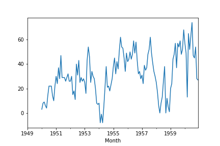
result=adfuller((df['Seasonal_Difference']).dropna())
dict(zip(['adf', 'pvalue', 'usedlag', 'nobs', 'critical' 'values', 'icbest'],result))
{'adf': -3.383020726492481,
 'pvalue': 0.011551493085514952,
 'usedlag': 1,
 'nobs': 130,
 'criticalvalues': {'1%': -3.4816817173418295,
  '5%': -2.8840418343195267,
  '10%': -2.578770059171598},
 'icbest': 919.527129208137}
The p-value is less than 0.05 thus it’s stationary and we don’t have to use differencing. That suggests to use 0 for the D value.
Autocorrelation and Partial Autocorrelation Plots (p,q and P,Q parameters)
The last step before the ARIMA model is to create the Autocorrelation and Partial Autocorrelation Plots to help us estimate the p,q, P, and Q parameters.
There are some very useful rules for ARIMA and Seasonal ARIMA models that we are using to help us estimate the parameters by looking at the Autocorrelation and Partial Autocorrelation Plots. We will create the plots for the second difference and the seasonal difference of our time series because these are the stationary series we end up using in ARIMA (d=2, D=0).
First, let’s plot ACF and PACF for the second difference.
from statsmodels.graphics.tsaplots import plot_acf, plot_pacf

fig1=plot_acf(df['2difference'].dropna())
fig2=plot_pacf(df['2difference'].dropna())

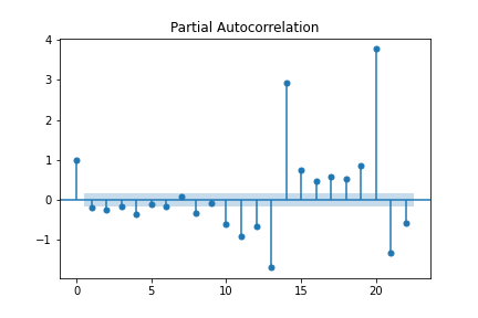
We can see that we have a sharp cut-off at lag-1 in both of our plots. According to the rules we mentioned above, this suggests using an AR and MA term. In other words, p=1 and q=1.
Now, we need the same plots of Seasonal Difference.
fig1=plot_acf(df['2difference'].dropna())
fig2=plot_pacf(df['2difference'].dropna())
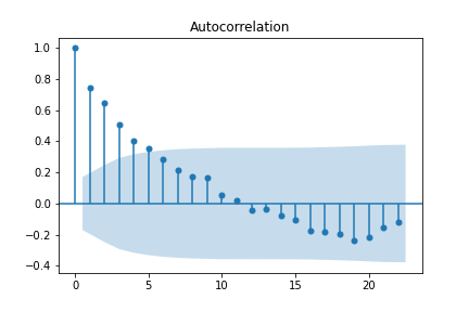

We have a gradual decrease in the Autocorrelation plot and a sharp cut-off in the Partial Autocorrelation plot. This suggests using AR and not over the value of 1 for the seasonal part of the ARIMA.
The values we chose may not be optimum. You can play around with these parameters to fine-tune the model having as a guide the rules we mentioned above.
The ARIMA Model
from statsmodels.tsa.statespace.sarimax import SARIMAX
model=SARIMAX(df['#Passengers'],order=(1,2,1),seasonal_order=(1, 0, 0, 12))
result=model.fit()
We can plot the residuals of the model to have an idea of how well the model is fitted. Basically, the residuals are the difference between the original values and the predicted values from the model.
result.resid.plot(kind='kde')

It’s time for a forecast. We will create some future dates to add them to our data so we can predict the future values.
from pandas.tseries.offsets import DateOffset
new_dates=[df.index[-1]+DateOffset(months=x) for x in range(1,48)]
df_pred=pd.DataFrame(index=new_dates,columns =df.columns)
df_pred.head()
The ARIMA model predicts taking as arguments the start and the end of the enumerated index and not the date range.
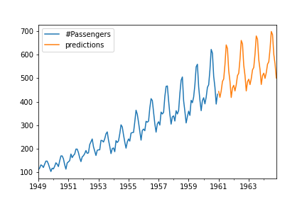
We created an empty data frame having indexes future dates and we concatenated them in our original data. Our data had 144 rows and the new dada we added have 48 rows. Therefore, to get the predictions only for the future data, we will predict from row 143 to 191.
df2=pd.concat([df,df_pred])


df2['predictions']=result.predict(start=143,end=191)
df2[['#Passengers','predictions']].plot()
Summing It Up
Arima is a great model for forecasting and It can be used both for seasonal and non-seasonal time series data.
For non-seasonal ARIMA you have to estimate the p, d, q parameters, and for Seasonal ARIMA it has 3 more that applies to seasonal difference the P, D, Q parameters.
The pipeline that we are using to run an ARIMA model is the following:
- Look at your time series to understand if they are Seasonal or Non-Seasonal.
- Apply differencing to time series and seasonal difference if needed to reach stationarity to get an estimate for d and D values.
- Plot the Autocorrelation and Partial Autocorrelation plots to help you estimate the p, P, and q, Q values.
- Fine-tune the model if needed changing the parameters according to the general rules of ARIMA
Useful links:
Rules for ARIMA
Arima In R
How To Backtest Your Crypto Trading Strategies In R
ARIMA in Wikipedia