

We will show how we can price the European Options with Monte Carlo simulation using R. Recall that the European options are a version of an options contract that limits execution to its expiration date. We will focus on the call and put options only. We assume that the reader is familiar with European Options and the Black Scholes formula.
Black-Scholes Formula
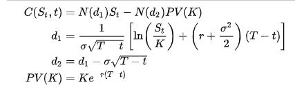
We can calculate the price of the European put and call options explicitly using the Black–Scholes formula.
Call Option
The value of a call option for a non-dividend-paying underlying stock in terms of the Black–Scholes parameters is:
Put Option
The price of a corresponding put option based on put–call parity is:
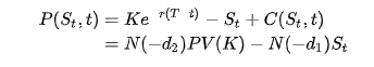
Where in both cases the notion is the following:
- N(.) is the cumulative distribution function of the standard normal distribution
- T-t is the time to maturity (expressed in years)
- St is the spot price of the underlying asset
- K is the strike price
- r is the risk-free rate (annual rate, expressed in terms of continuous compounding)
- σ is the volatility of returns of the underlying asset.
Pricing of European Options with Black-Scholes formula
We can easily get the price of the European Options in R by applying the Black-Scholes formula.
Scenario. Let’s assume that we want to calculate the price of the call and put option with:
- K: Strike price is equal to 100
- r: The risk-free annual rate is 2%
- sigma: The volatility σ is 20%
- T: time to maturity in years is 0.5
- S0: The current price is equal to 102
K = 100
r = 0.02
sigma = 0.2
T = 0.5
S0 = 102

# call option

d1 <- (log(S0/K) + (r + sigma^2/2) * T)/(sigma * sqrt(T))
d2 <- d1 - sigma * sqrt(T)
phid1 <- pnorm(d1)
call_price <- S0 * phid1 - K * exp(-r * T) * pnorm(d2)

# put option
d1 <- (log(S0/K) + (r + sigma^2/2) * T)/(sigma * sqrt(T))
d2 <- d1 - sigma * sqrt(T)
phimd1 <- pnorm(-d1)
put_price <- -S0 * phimd1 + K * exp(-r * T) * pnorm(-d2)

c(call_price, put_price)
[1] 7.288151 4.293135So the price of the call and put option is 7.288151 and 4.293135 respectively.
Pricing of European Options with Monte Carlo Simulation
Given the current asset price at time 0 is \(S_0\), then the asset price at time T can be expressed as:
\(S_T = S_0e^{(r- \frac{\sigma^2}{2})T + \sigma W_T}\)
where \(W_T\) follows the normal distribution with mean 0 and variance T. The pay-off of the call option is \(max(S_T-K,0)\) and for the put option is \(max(K-S_T)\).
Simple Monte Carlo
Let’s apply a simple Monte Carlo Simulation with 1M runs, where we will get the price and the standard error of the call and put option. As parameters, we will use the same as the example above.
# call put option monte carlo
call_put_mc<-function(nSim=1000000, tau, r, sigma, S0, K) {

  Z <- rnorm(nSim, mean=0, sd=1)
  WT <- sqrt(tau) * Z
  ST = S0*exp((r - 0.5*sigma^2)*tau + sigma*WT)

  # price and standard error of call option
  simulated_call_payoffs <- exp(-r*tau)*pmax(ST-K,0)
  price_call <- mean(simulated_call_payoffs)
  sterr_call <- sd(simulated_call_payoffs)/sqrt(nSim)

  # price and standard error of put option
  simulated_put_payoffs <- exp(-r*tau)*pmax(K-ST,0)
  price_put <- mean(simulated_put_payoffs)
  sterr_put <- sd(simulated_put_payoffs)/sqrt(nSim)


  output<-list(price_call=price_call, sterr_call=sterr_call,
               price_put=price_put, sterr_put=sterr_put)
  return(output)

}


set.seed(1)
results<-call_put_mc(n=1000000, tau=0.5, r=0.02, sigma=0.2, S0=102, K=100)

results
And we get:
$price_call
[1] 7.290738

$sterr_call
[1] 0.01013476

$price_put
[1] 4.294683

$sterr_put
[1] 0.006700902
As we can see, the estimated prices from the Monte Carlo Simulation are very close to those obtained from the Black-Scholes formula (7.290738 vs 7.288151 and 4.294683 vs 4.293135)
Antithetic Variates Method
The method of antithetic variates attempts to reduce variance by introducing negative dependence between pairs of replications. In a simulation driven by independent standard normal random variables, antithetic variates can be implemented by pairing a sequence Zl, Z2, .. . of standard normal variables with the sequence -Zl, -Z2, . ..of standard normal variables. If the Zi are used to simulate the increments of a Brownian path, then the – Zi simulate the increments of the reflection of the path about the origin. This again suggests that running a pair of simulations using the original path and then its reflection may result in lower variance. Note that the antithetic variates estimator is simply the average of all 2n observations. Let’s apply the “Antithetic Variates Method” and compare the results with the simple Monte Carlo.
Note that the pair for the call will be the:
\(( e^{-rT}max(S_{WT}-K,0), e^{-rT}max(S_{-WT}-K,0) )\)
and the estimated price will be the average of the pair for every simulation step.
antithetic_call_put_mc<-function(nSim, tau, r, sigma, S0, K) {

  Z <- rnorm(nSim, mean=0, sd=1)

  WT <- sqrt(tau) * Z
  # ST1 and ST2 and the antithetic variates
  ST1 = (S0*exp((r - 0.5*sigma^2)*tau + sigma*WT))
  ST2 = (S0*exp((r - 0.5*sigma^2)*tau + sigma*(-WT)))

  # call option price and standard error
  simulated_call_payoffs1 <- exp(-r*tau)*pmax(ST1-K,0)
  simulated_call_payoffs2 <- exp(-r*tau)*pmax(ST2-K,0)
  # get the average
  simulated_call_payoffs <- ( simulated_call_payoffs1 + simulated_call_payoffs2)/2
  price_call <- mean(simulated_call_payoffs)
  sterr_call <- sd(simulated_call_payoffs)/sqrt(nSim)


  # put option price and standard error
  simulated_put_payoffs1 <- exp(-r*tau)*pmax(K-ST1,0)
  simulated_put_payoffs2 <- exp(-r*tau)*pmax(K-ST2,0)
  # get the average
  simulated_put_payoffs <- (simulated_put_payoffs1+simulated_put_payoffs2)/2
  price_put <- mean(simulated_put_payoffs)
  sterr_put <- sd(simulated_put_payoffs)/sqrt(nSim)

  output<-list(price_call=price_call, sterr_call=sterr_call,
               price_put=price_put, sterr_put=sterr_put )
  return(output)

}

set.seed(1)
results<-antithetic_call_put_mc(n=1000000, tau=0.5, r=0.02, sigma=0.2, S0=102, K=100)

results
And we get:
$price_call
[1] 7.290193

$sterr_call
[1] 0.004993403

$price_put
[1] 4.294812

$sterr_put
[1] 0.003636479
We see that the estimated prices are again very close but the standard error is much much lower with the antithetic variates method compared to the simple Monte Carlo (0.004993403 vs 0.01013476 and 0.003636479 vs 0.006700902). Someone can argue that this variance reduction is due to the fact that by generating 1M pairs was like generating 2M simulations. We have to mention that computationally was not expensive to get the pairs because again we generated from the standard normal and the pair was consisting of the original value and of the original value with a different sign. However, we can run the simulation again half times, just for comparison.
set.seed(1)
results<-antithetic_call_put_mc(n=1000000/2, tau=0.5, r=0.02, sigma=0.2, S0=102, K=100)
results
$price_call
[1] 7.28989

$sterr_call
[1] 0.007057805

$price_put
[1] 4.294863

$sterr_put
[1] 0.005140888
As we can see, even if we run the half simulations, the standard error is lower than that of the simple Monte Carlo.
Importance Sampling Method
This is the idea of the importance sampling, is to try to give more weight to the “important” so that to increase sampling efficiency and as a result to reduce the standard error of the simulation. We will change the measure by considering the identical function I[ST>K] for the call options and I[ST<K] for the put option.
importance_call_put_mc<-function(nSim, tau, r, sigma, S0, K) {

  Z <- rnorm(nSim, mean=0, sd=1)
  WT <- sqrt(tau) * Z
  ST = S0*exp((r - 0.5*sigma^2)*tau + sigma*WT)

  # call option price and standard error
  simulated_call_payoffs <- (exp(-r*tau)*pmax(ST-K,0))[ST>K]
  price_call <- mean(simulated_call_payoffs*mean(ST>K))
  sterr_call <- sd(simulated_call_payoffs*mean(ST>K))/sqrt(nSim)


  # put option price and standard error
  simulated_put_payoffs <- (exp(-r*tau)*pmax(K-ST,0))[ST<K]
  price_put <- mean(simulated_put_payoffs*mean(ST<K))
  sterr_put <- sd(simulated_put_payoffs*mean(ST<K))/sqrt(nSim)


  output<-list(price_call=price_call, sterr_call=sterr_call,
               price_put=price_put, sterr_put=sterr_put )
  return(output)

}

set.seed(1)

results<-importance_call_put_mc(n=1000000, tau=0.5, r=0.02, sigma=0.2, S0=102, K=100)

results
And we get:
$price_call
[1] 7.290738

$sterr_call
[1] 0.005785042

$price_put
[1] 4.294683

$sterr_put
[1] 0.003114197
Again, we see that by applying the importance sampling technique, we got a very close estimation of the price and much lower standard error compared to the simple Monte Carlo Method.
Discussion
We showed how we can calculate the price of the European options explicitly by applying the Black-Scholes formula and we showed how we can estimate the prices by applying Monte Carlo simulation. Finally, we provided examples of advanced Monte Carlo techniques such as the antithetic variates and the importance sampling which have as a result a more effective simulation with lower standard error.


10 thoughts on “Pricing of European Options with Monte Carlo”
George,
Nice blog post! However, I recommend you take another look at the importance sampling part of it. The current version is not doing quite what you think it’s doing.
Firstly, please check line 27 of the code where the function call isn’t what you meant so the results shown in the blog post are those previously calculated in the antithetic discussion.
Secondly (and more importantly), you aren’t actually doing importance sampling so the results of your “importance sampling” calculation are actually identical to those of the simple Monte Carlo. (The standard error calculation is incorrect — you will get the same standard error as in the simple case.)
The pmax() in the simple MC payoff calculation makes sure you sum up the payoffs only from the cases where (for the call option) ST>K and the mean() divides that sum by the total number of simulated prices. In the “importance sampling” case , the mean() is again summing over only those cases and dividing by the number of cases where ST>K. However, mean(ST>K) gives the fraction of cases where ST>K so multiplying by this effectively adjusts the denominator to again be the total number of simulated prices. For example, if you ran 1 million cases and 500,000 of them had ST>K (so the fraction of cases where ST>K is 1/2), both calculations sum up the payoffs from the 500,000 positive payoff cases and the simple MC would then divide that by 1 million while the “importance sampling” calculation instead multiplies by 1/2 and divides that by 500,000.
Rich
PS: Still a nicely written, worthwhile blog post.
Thank you Rich for your comments. Yes there was a typo in line 27 where I was calling the previous function. I ran again the “Importance Sampling” and the StDev appears to be lower than the simple Monte Carlo. Can you please share the right script for the Importance Sampling for the European Options?
The standard error formulas for the “simple” MC function also apply to your “importance sampling” function because *they are doing the exact same calculation*. For example, here is code running each one multiple times and computing the std error based on the samples. (I run 100 simulations of 10,000 draws each which corresponds to your single 1 million simulation draw run.) If you run it with your functions, you will see that both functions estimate the call value with identical standard error.
“`
# compute mean and sd for “simple” MC function (call price)
set.seed(1)
nTest = 100
res = numeric(nTest)
for (i in 1:nTest){
res[i] = call_put_mc(n=10000, tau=0.5, r=0.02, sigma=0.2, S0=102, K=100)$price_call
}
mean(res); sd(res)
set.seed(1)
# compare with outputs from the function
results = call_put_mc(n=1000000, tau=0.5, r=0.02, sigma=0.2, S0=102, K=100)
results[1:2]
# compute mean and sd for “importance sampling” function (call price)
set.seed(1)
nTest = 100
res = numeric(nTest)
for (i in 1:nTest){
res[i] = importance_call_put_mc(n=10000, tau=0.5, r=0.02, sigma=0.2, S0=102, K=100)$price_call
}
mean(res); sd(res)
# compare with outputs from the function
set.seed(1)
results = importance_call_put_mc(n=1000000, tau=0.5, r=0.02, sigma=0.2, S0=102, K=100)
results[1:2]
“`
Sorry, the comparison run of the function should be with n=10000 to match the standard errors. (Not sure how to edit a comment — maybe you can make the change and delete this one. Thanks!)
To carry out importance sampling, you need to sample with a different probability distribution which gives more weight where it is needed. Here is an example for the call option where Z values high enough to have positive payoffs are sampled with an exponential distribution (which decays more slowly than the normal distribution thereby giving more weight to large Z outcomes). If you try it with high strike prices (e.g. K = 120), you will see that it has much lower standard error than the “simple” MC case.
“`
# Use importance sampling to simulate call value
importance_call_mc<-function(nSim, tau, r, sigma, S0, K) {
# compute minimum Z draw for positive payoffs
Zmin = log(K/S0/exp((r – 0.5*sigma^2)*tau))/sigma/sqrt(tau)
# importance sample with exponential distrib above Zmin for Z
Z = Zmin + rexp(nSim, rate = 1)
# sample weight is normal density divided by the exponential distrib
sample_weights = exp(-0.5*Z^2 + Z – Zmin)/sqrt(2.*pi)
# estimate call option price as weighted expected payoff
WT <- sqrt(tau) * Z
ST = S0 * exp((r – 0.5*sigma^2) * tau + sigma * WT)
simulated_call_payoffs <- exp(-r * tau) * pmax(ST – K, 0)
price_call <- mean(simulated_call_payoffs * sample_weights)
output<-list(price_call=price_call)
return(output)
}
# compute mean and sd for importance sampling function (call price)
set.seed(1)
nTest = 100
res = numeric(nTest)
for (i in 1:nTest){
res[i] = importance_call_mc(n=10000, tau=0.5, r=0.02, sigma=0.2, S0=102, K=100)$price_call
}
mean(res); sd(res)
“`
Thank you Rich for your time and for your response. My 5 cents:
1) When you call the function you should change the n to nSim
2) The StDev should be derived from the nSim. As I see here, you derive the StDev by considering the nSim each time
3) For this example, the price should be around 7.29 and I get 7.22 (set.seed(1); importance_call_mc(nSim =10000, tau=0.5, r=0.02, sigma=0.2, S0=102, K=100))
1) You are correct that the n should be nSim (but R still matches correctly with n R function calls use partial argument matching).
2) Yes, it is better is to do the math and derive it. I was lazy and just ran the simulation many times to compute it numerically.
3) When I copy the code from the comment and run it (after fixing the characters that HTML messed up) I get the following:
[1] 7.288323
[1] 0.06543349
Thank you Rich. The StDev that you calculate is from the average of the nSims. You need to derive the Mean and the StDev within the function. What you were doing is to run 100 times the 10000 simulations.
Hi George,
Thank you for this nice post! I would like to ask how you would incorporate a threshold into the calculation of the put payoffs? For example, let’s say S0 = 100 and the put becomes worthless once the stock price falls below 75, so the payoff at maturity of this put option is 0 if the price falls below 75 any time.
Thank you in advance!
Hi Marton,
You need to add this condition to the Monte Carlo simulation