Meta Analysis in R

Introduction

We can analyze different scientific studies that address the same question by applying a meta-analysis. The assumption is that every individual study contains some degree of error. For example, a study could be the mortality rate of two treatments for a specific disease. The goal is to obtain pooled summary estimates from individual studies by taking into consideration the heterogeneity among individual studies. The aggregated data from the individual studies leads to higher statistical power.

Procedure

• Define the research question
• Define inclusion/exclusion criteria for individual studies screened
• Search literature
• Select eligible studies
• Collect data
• Aggregate findings across studies and obtain pooled estimates of effect size
• Evaluate heterogeneity of included studies
• Conduct sensitivity and subgroup analyses

Statistical Models

• Pool effect sizes (of individual studies) into one overall effect
• Two types of statistical models to combine data, Fixed Effect Model and Random Effects Model
• Frequentist vs Bayesian approach

Example of Meta Analysis in R

We will provide an example of Meta Analysis in R using the meta library. Let’s start.

library(meta)
data("Fleiss1993cont")

head(Fleiss1993cont)

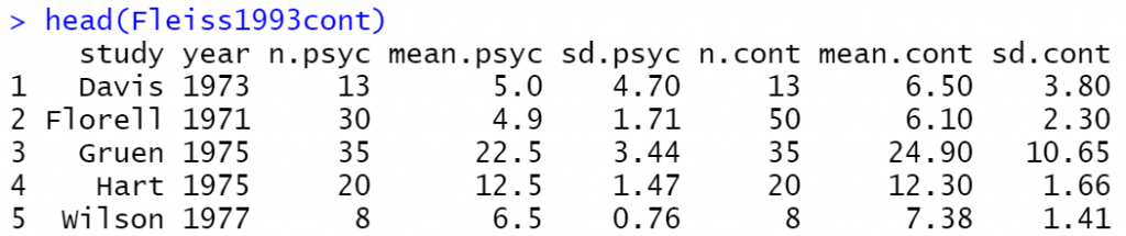
We will work with the Fleiss1993cont dataset where:

study	study label
year	year of publication
n.psyc	number of observations in psychotherapy group
mean.psyc	estimated mean in psychotherapy group
sd.psyc	standard deviation in psychotherapy group
n.cont	number of observations in control group
mean.cont	estimated mean in control group
sd.cont	standard deviation in control group

# meta-analysis with continuout outcome
# comb.fixed/comb.random: indicator whether a fix/random effect mata-analysis to be conducted.
# sm: Three different types of summary measures to choose,standardized mean difference (SMD),mean difference (MD), ratio of means (ROM)
res.flesiss =  metacont(n.psyc, mean.psyc, sd.psyc, 
                        n.cont, mean.cont, sd.cont,
                        comb.fixed = T, comb.random = T, studlab = study,
                        data = Fleiss1993cont, sm = "SMD") 
res.flesiss

Output

            SMD             95%-CI %W(fixed) %W(random)
Davis   -0.3399 [-1.1152;  0.4354]      11.5       11.5
Florell -0.5659 [-1.0274; -0.1044]      32.6       32.6
Gruen   -0.2999 [-0.7712;  0.1714]      31.2       31.2
Hart     0.1250 [-0.4954;  0.7455]      18.0       18.0
Wilson  -0.7346 [-1.7575;  0.2883]       6.6        6.6

Number of studies combined: k = 5
Number of observations: o = 232

                         SMD             95%-CI     z p-value
Fixed effect model   -0.3434 [-0.6068; -0.0800] -2.56  0.0106
Random effects model -0.3434 [-0.6068; -0.0800] -2.56  0.0106

Quantifying heterogeneity:
 tau^2 = 0 [0.0000; 0.6936]; tau = 0 [0.0000; 0.8328]
 I^2 = 0.0% [0.0%; 79.2%]; H = 1.00 [1.00; 2.19]

Test of heterogeneity:
    Q d.f. p-value
 3.68    4  0.4515

Details on meta-analytical method:
- Inverse variance method
- DerSimonian-Laird estimator for tau^2
- Jackson method for confidence interval of tau^2 and tau
- Hedges' g (bias corrected standardised mean difference)

Forest

forest(res.flesiss, leftcols = c('studlab'))

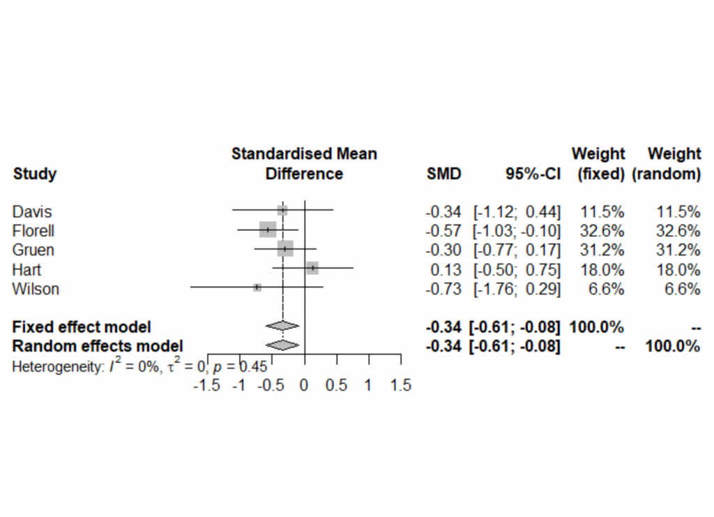
• According to the pooled results of meta-analysis, both fixed and random effects models yield a significant benefit of the intervention group against the control group (for the days of hospital stay, the lower, the better).
• The p-value =0.45 for the Cochran’s Q test, indicating no heterogeneity.

Funnel Plot

funnel(res.flesiss)

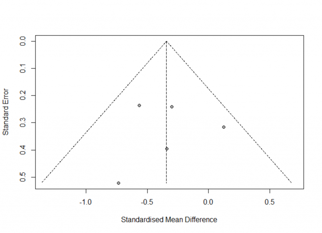
• metabias: Test for funnel plot asymmetry, based on rank correlation or linear regression method.
• Use Egger’s test to check publication bias, can take string ‘Egger’ or ‘linreg’.

metabias(res.flesiss, method.bias = 'linreg', k.min = 5, plotit = T)

Output

Linear regression test of funnel plot asymmetry

Test result: t = -0.04, df = 3, p-value = 0.9730

Sample estimates:
    bias se.bias intercept se.intercept
 -0.0668  1.8154   -0.3241       0.5455

Details:
- multiplicative residual heterogeneity variance (tau^2 = 1.2251)
- predictor: standard error
- weight:    inverse variance
- reference: Egger et al. (1997), BMJ

The p-value is 0.973 which implies no publication bias. However, this meta-analysis contains k=5 studies. Egger’s test may lack the statistical power to detect bias when the number of studies is small (i.e., k<10).

Binary case

At this point, we will provide an example by taking into consideration a binary case.

load("binarydata.RData")
binarydata

• Author: This signifies the column for the study label (i.e., the first author)
• Ee: Number of events in the experimental treatment arm
• Ne: Number of participants in the experimental treatment arm
• Ec: Number of events in the control arm
• Nc: Number of participants in the control arm

The Analysis:

• Use metabin to do the calculation.
• As we want to have a pooled effect for binary data, we have to choose another summary measure now. We can choose from “OR” (Odds Ratio), “RR” (Risk Ratio), or RD (Risk Difference), among other things.
• method: indicating which method is to be used for pooling of studies.

m.bin <- metabin(Ee,Ne,Ec,Nc,
                 data = binarydata,
                 studlab = paste(Author),
                 comb.fixed = T,comb.random = T,
                 method = 'MH',sm = "RR") # Mantel Haenszel weighting

Output

                        RR           95%-CI %W(fixed) %W(random)
Alcorta-Fleischmann 0.5018 [0.0462; 5.4551]       1.4        1.4
Craemer             1.0705 [0.5542; 2.0676]      15.2       18.9
Eriksson            1.1961 [0.3657; 3.9124]       4.5        5.8
Jones               0.5286 [0.1334; 2.0945]       5.3        4.3
Knauer              0.3278 [0.0134; 8.0140]       1.4        0.8
Kracauer            0.9076 [0.3512; 2.3453]       8.0        9.1
La Sala             0.9394 [0.4233; 2.0847]      11.2       12.9
Maheux              0.0998 [0.0128; 0.7768]       9.0        1.9
Schmidthauer        0.7241 [0.2674; 1.9609]       7.9        8.3
van der Zee         0.8434 [0.4543; 1.5656]      18.5       21.4
Wang                0.5519 [0.2641; 1.1534]      17.5       15.1

Number of studies combined: k = 11
Number of observations: o = 17604
Number of events: e = 194

                         RR           95%-CI     z p-value
Fixed effect model   0.7536 [0.5696; 0.9972] -1.98  0.0478
Random effects model 0.7885 [0.5922; 1.0499] -1.63  0.1038

Quantifying heterogeneity:
 tau^2 = 0; tau = 0; I^2 = 0.0% [0.0%; 60.2%]; H = 1.00 [1.00; 1.59]

Test of heterogeneity:
    Q d.f. p-value
 7.29   10  0.6976

Details on meta-analytical method:
- Mantel-Haenszel method
- DerSimonian-Laird estimator for tau^2
- Mantel-Haenszel estimator used in calculation of Q and tau^2 (like RevMan 5)
- Continuity correction of 0.5 in studies with zero cell frequencies

Forest

forest(m.bin, leftcols = c('studlab'))

funnel(m.bin)
metabias(m.bin, method.bias = 'linreg', plotit = T)

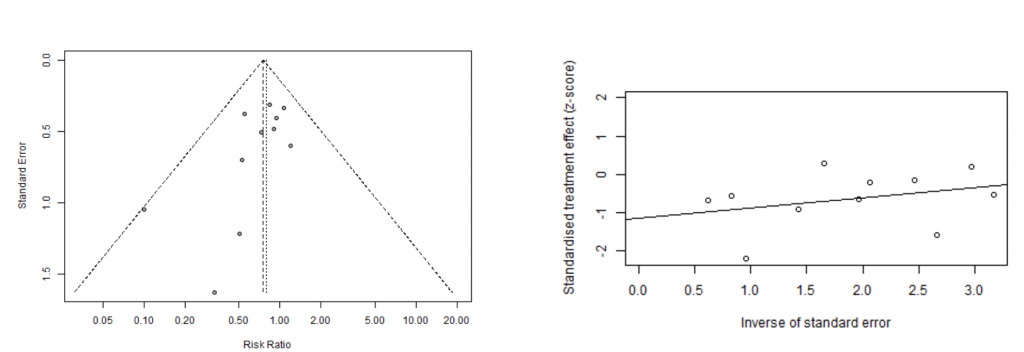
Linear regression test of funnel plot asymmetry

Test result: t = -2.05, df = 9, p-value = 0.0701

Sample estimates:
    bias se.bias intercept se.intercept
 -1.1286  0.5493    0.2623       0.2661

Details:
- multiplicative residual heterogeneity variance (tau^2 = 0.5443)
- predictor: standard error
- weight:    inverse variance
- reference: Egger et al. (1997), BMJ

Limitations

The limitation of Meta Analysis is that it can only conduct pariwise comparisions, and cannot include multi-arm trials.

References

[1] Dr. Na Zhao