
Using R and the anova function we can easily compare nested models. Where we are dealing with regression models, then we apply the F-Test and where we are dealing with logistic regression models, then we apply the Chi-Square Test. By nested, we mean that the independent variables of the simple model will be a subset of the more complex model. In essence, we try to find the best parsimonious fit of the data. Note that we should fit the models on the same dataset.
The Null Hypothesis is that the simple model is better and we reject the null hypothesis if the p-value is less than 5% inferring that the complex model is is significantly better than the simple one.
Example of Comparing Nested Models
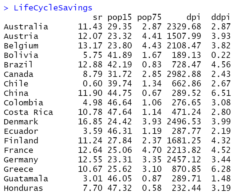
Let’s work with the LifeCycleSavings dataset by considering as dependent variable the sr and the rest as independent variables (IV).
Let’s say that we want to compare the following two models:
fit0which is the \(sr = \alpha\)fit1which is the \(sr = \alpha +\beta \times pop15\)
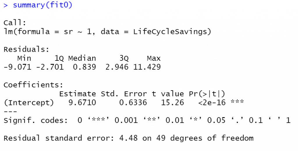
fit0 <- lm(sr ~ 1, data = LifeCycleSavings)

fit1 <- lm(sr ~ pop15, data = LifeCycleSavings)


summary(fit0)
summary(fit1)
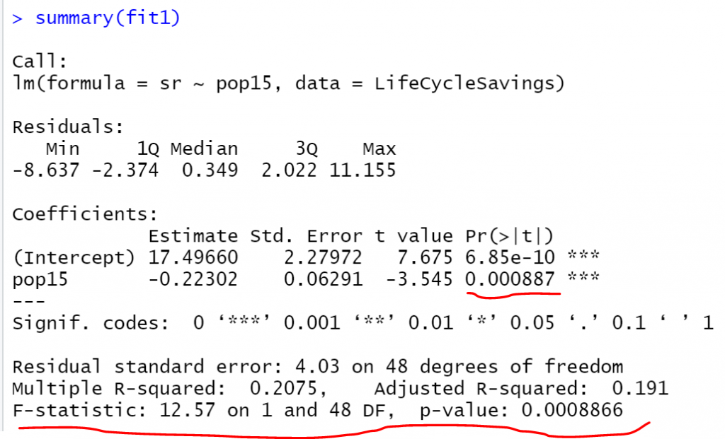
Notice the P-value of the F-Test of the fit1 model is 0.0008866 which actually tests the Null Hypothesis that “all the beta coefficients are zero” versus the alternative hypothesis that “at least one beta coefficient is not zero”. Since we have only one beta coefficient, the pop15 the p-value of the F-Test is the same as the p-value of the T-Test as we can see above.
Now, if we compare the fit0 vs the fit1, in essence, we test if we should include the pop15 coefficient or not, thus we expect to get the same p-value. Let’s compare the nested models using anova:
anova(fit0, fit1, test='F')
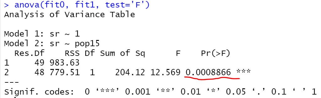
As expected we got the same p-value, and we can say that we should prefer the fit1 compared to fit0 model.
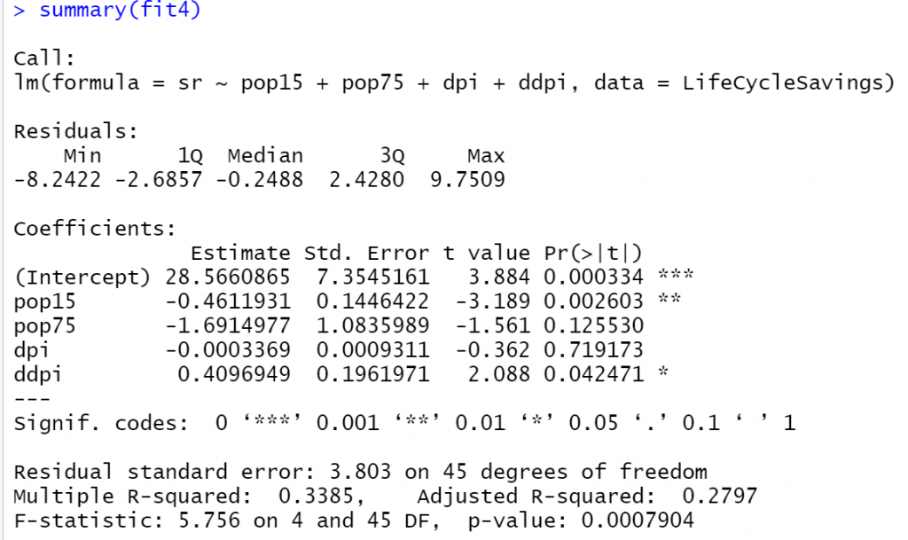
Let’s make another comparison by comparing the fit1 compared to the fit4 which contains all the IVs.
fit4<-lm(sr~pop15+pop75+dpi+ddpi, data = LifeCycleSavings)

summary(fit4)
Let’s compare the two models:
anova(fit1, fit4, test='F')

The p-value is 0.04177 forcing us to reject the null hypothesis that the fit1 models is better. Finally, let’s compare the fit1 model versus the fit3 which contains the first 3 IV of the dataset.
fit3<-lm(sr~pop15+pop75+dpi, data = LifeCycleSavings)
anova(fit1, fit3, test='F')
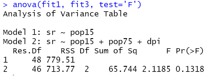
In this case, the p-value is 0.1318 which means that we should accept the null hypothesis that the fit1 is better than the fit3.