Get Started with Tensorflow 2.0 and CNN

In this tutorial we will show how you easily build a Convolutional Neural Network in Python and Tensorflow 2.0. We will work with the Fashion MNIST Dataset.

First things first, make sure that you have installed the 2.0 version of tensorflow:

import tensorflow as tf
print(tf.__version__)

2.0.0

Load the Data

We will load all the required libraries and we will load the fashion_mnist_data which is provided by tensorflow.

import tensorflow as tf
from tensorflow.keras.models import Sequential
from tensorflow.keras.layers import Dense, Flatten, Conv2D, MaxPooling2D
from tensorflow.keras.preprocessing import image
import matplotlib.pyplot as plt
import numpy as np
import pandas as pd

# Load the Fashion-MNIST dataset

fashion_mnist_data = tf.keras.datasets.fashion_mnist
(train_images, train_labels), (test_images, test_labels) = fashion_mnist_data.load_data()

# Print the shape of the training data

print(train_images.shape)
print(train_labels.shape)

The shape of the train and images and labels is:

(60000, 28, 28)
(60000,)

Let’s also define the labels

# Define the labels

labels = [
    'T-shirt/top',
    'Trouser',
    'Pullover',
    'Dress',
    'Coat',
    'Sandal',
    'Shirt',
    'Sneaker',
    'Bag',
    'Ankle boot'
]

Rescale the images to take values between 0 and 1.

# Rescale the image values so that they lie in between 0 and 1.
train_images = train_images/255.0
test_images = test_images/255.0

Display the first image:

# Display one of the images

i = 0
img = train_images[i,:,:]
plt.imshow(img)
plt.show()
print(f'label: {labels[train_labels[i]]}')

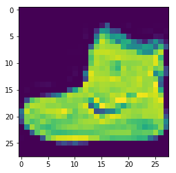
label: Ankle boot

Build the Model

The model will be a 2D Convolutional kernel (3 X 3) of 16 channels and relu activation. Then we will continue with a Max Pooling (3 x 3) and finally will be a fully connected layer of 10 neurons (as many as the labels) and a softmax activation function.

model = Sequential([
    Conv2D(16, (3,3), activation='relu', input_shape=(28,28,1)),
    MaxPooling2D((3,3)),
    Flatten(),
    Dense(10, activation='softmax')
])

# Print the model summary

model.summary()

Model: "sequential_1"
_________________________________________________________________
Layer (type)                 Output Shape              Param #   
=================================================================
conv2d_2 (Conv2D)            (None, 26, 26, 16)        160       
_________________________________________________________________
max_pooling2d_1 (MaxPooling2 (None, 8, 8, 16)          0         
_________________________________________________________________
flatten_3 (Flatten)          (None, 1024)              0         
_________________________________________________________________
dense_11 (Dense)             (None, 10)                10250     
=================================================================
Total params: 10,410
Trainable params: 10,410
Non-trainable params: 0

Compile the Model

We will compile the model using the adam optimizer and a sparse_categorical_crossentropy loss function. Finally, our metric will be the accuracy.

NB: We use the sparse_categorical_crossentropy because our y labels are in 1D array taking values from 0 to 9. If our y was labeled with one hot encoding then we would have used the categorical_crossentropy.

model.compile(optimizer='adam', #sgd etc
             loss='sparse_categorical_crossentropy',
             metrics=['accuracy'])

Fit the Model

Before we fit the model, we need to change the dimensions of the train images using the np.newaxis. Notice that from (60000, 28, 28) it will become (60000, 28, 28, 1)

train_images[...,np.newaxis].shape

(60000, 28, 28, 1)

We will run only 8 epochs (you can run more) and we will use a batch size equal to 256.

# Fit the model

history = model.fit(train_images[...,np.newaxis], train_labels, epochs=8, batch_size=256)

Train on 60000 samples
Epoch 1/8
60000/60000 [==============================] - 51s 858us/sample - loss: 1.2626 - accuracy: 0.6541
Epoch 2/8
60000/60000 [==============================] - 51s 843us/sample - loss: 1.0360 - accuracy: 0.6748
Epoch 3/8
60000/60000 [==============================] - 50s 835us/sample - loss: 0.9219 - accuracy: 0.6908
Epoch 4/8
60000/60000 [==============================] - 50s 837us/sample - loss: 0.8543 - accuracy: 0.7028
Epoch 5/8
60000/60000 [==============================] - 50s 837us/sample - loss: 0.8096 - accuracy: 0.7139
Epoch 6/8
60000/60000 [==============================] - 49s 823us/sample - loss: 0.7762 - accuracy: 0.7214
Epoch 7/8
60000/60000 [==============================] - 52s 858us/sample - loss: 0.7496 - accuracy: 0.7292
Epoch 8/8
60000/60000 [==============================] - 49s 825us/sample - loss: 0.7284 - accuracy: 0.7357

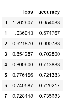
Get the training history

# Load the history into a pandas Dataframe

df = pd.DataFrame(history.history)
df

Evaluate the model 

We will evaluate our model on the test dataset.

# Evaluate the model

model.evaluate(test_images[...,np.newaxis], test_labels, verbose=2)

10000/1 - 6s - loss: 0.5551 - accuracy: 0.7299

As we can see, the accuracy of the test dataset is 0.7299.

Make Predictions

Finally, let’s see how we can get predictions.

# Choose a random test image

random_inx = np.random.choice(test_images.shape[0])

test_image = test_images[random_inx]
plt.imshow(test_image)
plt.show()
print(f"Label: {labels[test_labels[random_inx]]}")

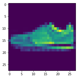
# Get the model predictions

predictions = model.predict(test_image[np.newaxis,...,np.newaxis])
print(f'Model Prediction: {labels[np.argmax(predictions)]}')

And we get that this image is a Sneaker!

Model Prediction: Sneaker

Takeaway

That was an example of how we can start with TensorFlow and CNNs by building a decent model in a few lines of code. The images were on grace-scale (not RGB) but the logic is the same since we expanded the dimensions. We can try other architectures playing with the convolutional kernels, pooling, layers, regularization, optimizers, epochs, batch sizes, learning rates and so on.