Beginners Guide: Predict the Stock Market

We will show you how you can create a model capable of predicting stock prices. Our way to do it is by using historical data and more specifically, the closing prices of the last 10 days of the Stock.

Warning: Stock market prices are highly unpredictable. This project is entirely intended for research purposes! Don’t put any money on it!

To get our data we will use the Yahoo! Finance Market Downloader. For our first prediction we will get the TESLA stock.

import pandas as pd
import yfinance as yf
import datetime
import numpy as np

df=yf.download('TSLA',start='2020-01-07',  end='2021-01-07',progress=False)[['Close']]
df.head()

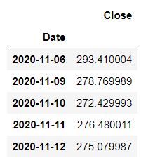
We only need the column Close that is the value that we want to predict. Our goal now is to transform the data so we can feed them into our Machine Learning model. We want to have as features the last 10 closing prices. The easiest way to do it is to use the shift function of Pandas.

df=pd.concat([df, df.shift(), df.shift(2),df.shift(3),df.shift(4),df.shift(5),
           df.shift(6),df.shift(7),df.shift(8),df.shift(9),df.shift(10)], axis=1).dropna()

df.columns=list(range(0,11))
df.rename(columns={0:'actual_stock_price'},inplace=True)

Predicting The Stock Price Of Next Day

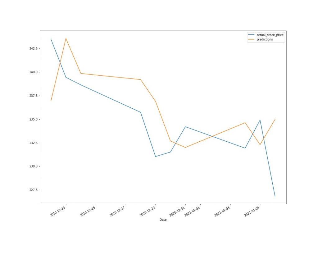
Firstly we will keep the last 10 days to compare the prediction with the actual value. For this method, we will predict the price of the next day and that means that we will use the actual stock price and not the predicted to compute the next days of the Test.

#split data into train and test. We will try to predict the last 10 days

train=df.head(len(df)-10)
test=df.tail(10)

from sklearn.linear_model import LinearRegression
lr=LinearRegression()
lr.fit(train[list(range(1,11))],train['actual_stock_price'])

test['predictions']=lr.predict(test[list(range(1,11))])

ax=test[['actual_stock_price','predictions']].plot(figsize=(15,12))

Predicting The Stock Price Of Next 10 Days

In this method we will predict the next 10 days of the price. That means that we will use our prediction to continue and predict the next days.

A very handy hack is that we can add days with DateTime. In this code, I’m making the prediction and I’m concatenating the new prediction to the Train Dataset as the next day. Then using a for loop I’m doing the same 10 times. Let’s see how it works by adding a new value to our train dataset. We will add the value of 100.

df=yf.download('TSLA',start='2020-01-07',  end='2021-01-07',progress=False)[['Close']]
train=df.head(len(df)-10)
test=df.tail(10)

train =pd.concat([train ,pd.DataFrame( {'Close':100},index=[train.tail(1).index[0]+datetime.timedelta(days=1)])])
train.tail()

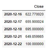
As you can see the new value is added in the dataset having as index the next day of 2020-12-21. Using this code we will now predict the next 10 days. Let’s see how it goes.

df=yf.download('TSLA',start='2020-01-07',  end='2021-01-07',progress=False)[['Close']]

train=df.head(len(df)-10)
test=df.tail(10)

predictions=[]
for i in range(0,10):
    x=pd.concat([train, train.shift(), train.shift(2),train.shift(3),train.shift(4),train.shift(5),
               train.shift(6),train.shift(7),train.shift(8),train.shift(9)], axis=1).dropna().tail(1)
    x.columns=range(1,11)
    pred=lr.predict(x)

    predictions.append(pred[0])
    train =pd.concat([train ,pd.DataFrame( {'Close':pred},index=[train.tail(1).index[0]+datetime.timedelta(days=1)])])
    
test['predictions']=predictions

test.plot(figsize=(15,12))

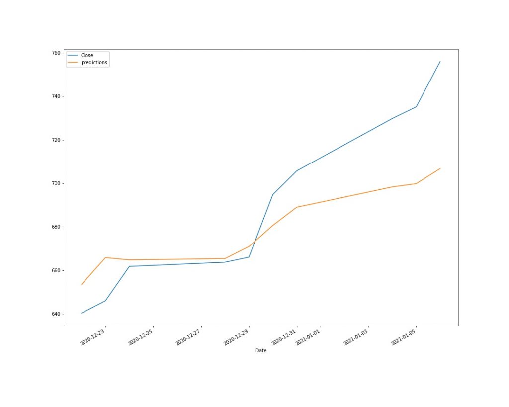
Not bad, right? This was just a simple example of how we can predict stock price by transforming a bit of the data and using a simple Linear Regression. We can learn a lot, so start to experiment with it! If you want to feel like the Wolf of Wall Street, you can test your model using virtual money.

BONUS: “Predict The Stock Market” Function

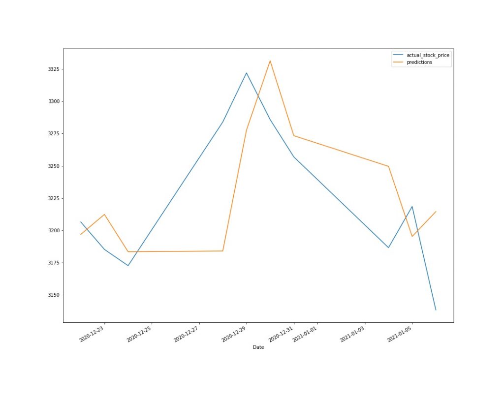
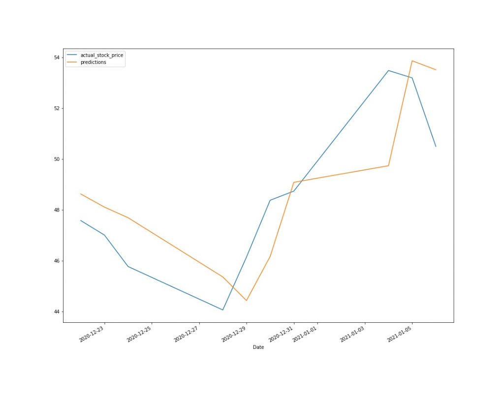
Let’s create a function with our first method and see how our model goes on some other stocks.

def predictnextday(symbol):
    df=yf.download(symbol,start='2020-01-07',  end='2021-01-07',progress=False)[['Close']]
    df=pd.concat([df, df.shift(), df.shift(2),df.shift(3),df.shift(4),df.shift(5),
               df.shift(6),df.shift(7),df.shift(8),df.shift(9),df.shift(10)], axis=1).dropna()

    df.columns=list(range(0,11))
    df.rename(columns={0:'actual_stock_price'},inplace=True)
    train=df.head(len(df)-10)
    test=df.tail(10)

    from sklearn.linear_model import LinearRegression
    lr=LinearRegression()
    lr.fit(train[list(range(1,11))],train['actual_stock_price'])

    test['predictions']=lr.predict(test.tail(10)[list(range(1,11))])

    ax=test[['actual_stock_price','predictions']].plot(figsize=(15,12))
    return(ax)

AMZN

NIO

PAYPAL