How to Predict Stock Prices with LSTM

In a previous post, we explained how to predict the stock prices using machine learning models. Today, we will show how we can use advanced artificial intelligence models such as the Long-Short Term Memory (LSTM). In previous post, we have used the LSTM models for Natural Language Generation (NLG) models, like the word based and the character based NLG models.

The LSTM Model

Long short-term memory (LSTM) is an artificial recurrent neural network (RNN) architecture used in the field of deep learning having feedback connections. Not only can process single data points such as images, but also entire sequences of data such as speech or video. For example, LSTM is applicable to tasks such as unsegmented, connected handwriting recognition, speech recognition, machine translation, anomaly detection, time series analysis etc.

The LSTM models are computationally expensive and require many data points. Usually, we train the LSTM models using GPU instead of CPU. Tensorflow is a great library for training LSTM models.

LSTM model for Stock Prices

Get the Data

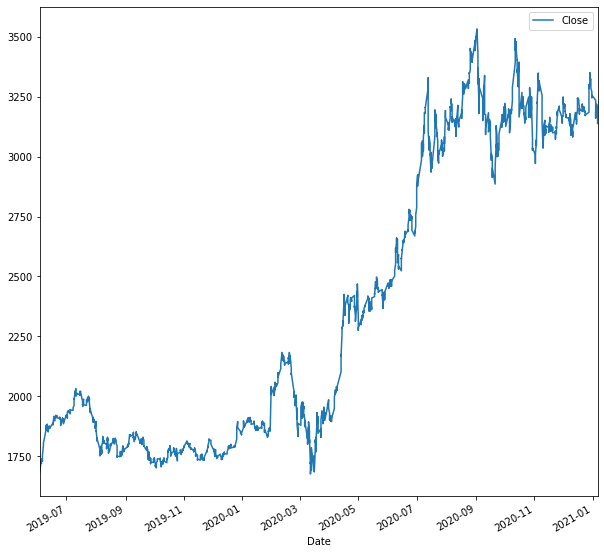
We will build an LSTM model to predict the hourly Stock Prices. The analysis will be reproducible and you can follow along. First, we will need to load the data. We will take as an example the AMZN ticker, by taking into consideration the hourly close prices from ‘2019-06-01‘ to ‘2021-01-07‘

import yfinance as yf
import pandas as pd
import numpy as np
from keras.models import Sequential
from keras.layers import Dense
from keras.layers import LSTM
from sklearn.preprocessing import MinMaxScaler
import matplotlib.pyplot as plt
%matplotlib inline  


data=yf.download('AMZN',start='2019-06-01', interval='1h',  end='2021-01-07',progress=False)[['Close']]
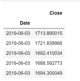
data.head()
 
data.plot(figsize=(10,10))
 

Prepare the Data

Our train data will have as features the look back values, which are the lag values noted as ‘lb’. For this example, we set the lb equal to 10. Notice that we scale the data on the “train” dataset using the MinMaxScaler() from scikit-learn. Finally, for this example, we keep as train dataset the first 90% of the observations and as a test dataset the rest 10%

cl = data.Close.astype('float32')
train = cl[0:int(len(cl)*0.80)]
scl = MinMaxScaler()
#Scale the data
scl.fit(train.values.reshape(-1,1))
cl =scl.transform(cl.values.reshape(-1,1))
#Create a function to process the data into lb observations look back slices
# and create the train test dataset (90-10)
def processData(data,lb):
    X,Y = [],[]
    for i in range(len(data)-lb-1):
        X.append(data[i:(i+lb),0])
        Y.append(data[(i+lb),0])
    return np.array(X),np.array(Y)


lb=10
X,y = processData(cl,lb)
X_train,X_test = X[:int(X.shape[0]*0.90)],X[int(X.shape[0]*0.90):]
y_train,y_test = y[:int(y.shape[0]*0.90)],y[int(y.shape[0]*0.90):]
print(X_train.shape[0],X_train.shape[1])
print(X_test.shape[0], X_test.shape[1])
print(y_train.shape[0])
print(y_test.shape[0])
 

Output:

2520 10
281 10
2520
281

Build the LSTM Model

We will work with the following LSTM Model.

#Build the model
model = Sequential()
model.add(LSTM(256,input_shape=(lb,1)))
model.add(Dense(1))
model.compile(optimizer='adam',loss='mse')

#Reshape data for (Sample,Timestep,Features) 
X_train = X_train.reshape((X_train.shape[0],X_train.shape[1],1))
X_test = X_test.reshape((X_test.shape[0],X_test.shape[1],1))

#Fit model with history to check for overfitting
history = model.fit(X_train,y_train,epochs=300,validation_data=(X_test,y_test),shuffle=False)

model.summary() 
 

Output:

Model: "sequential_33"
_________________________________________________________________
Layer (type)                 Output Shape              Param #   
=================================================================
lstm_51 (LSTM)               (None, 256)               264192    
_________________________________________________________________
dense_29 (Dense)             (None, 1)                 257       
=================================================================
Total params: 264,449
Trainable params: 264,449
Non-trainable params: 0
_________________________________________________________________

Predictions

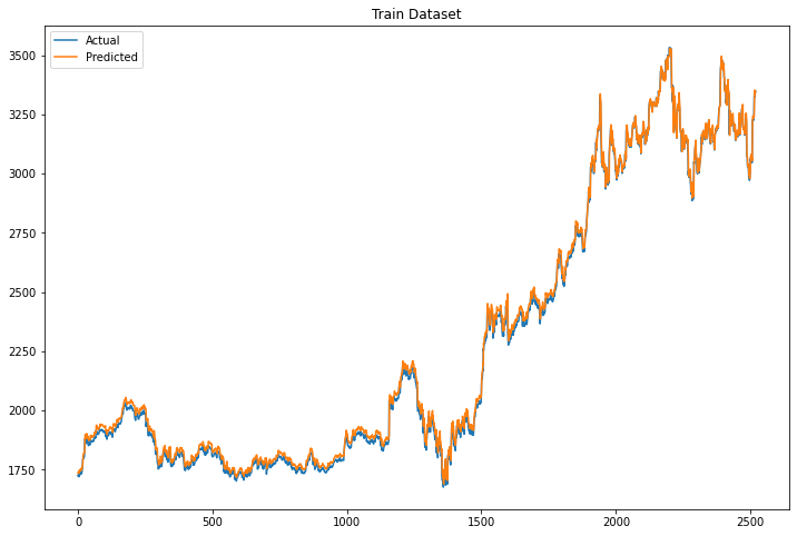
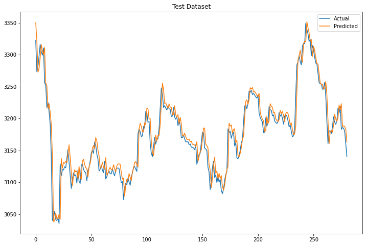
Let’s get the predictions on the train and test dataset:

Train

plt.figure(figsize=(12,8))

Xt = model.predict(X_train)
plt.plot(scl.inverse_transform(y_train.reshape(-1,1)), label="Actual")
plt.plot(scl.inverse_transform(Xt), label="Predicted")
plt.legend()
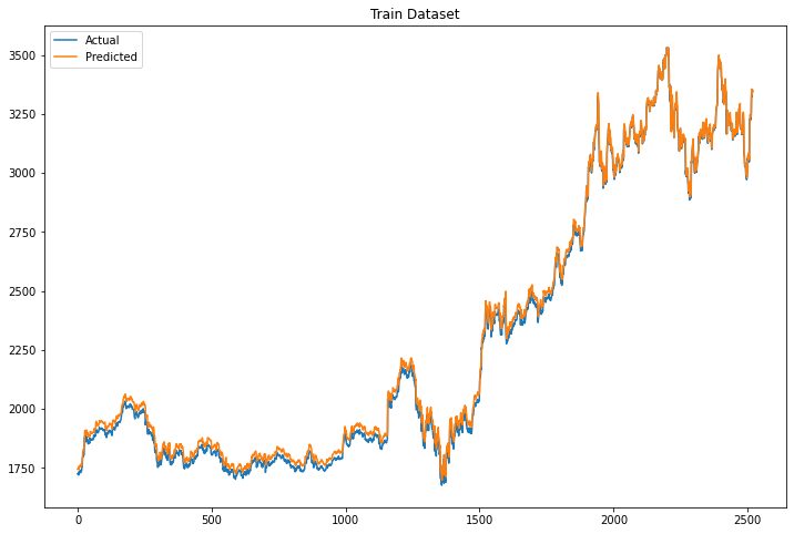
plt.title("Train Dataset")
 

Test

plt.figure(figsize=(12,8))
Xt = model.predict(X_test)
plt.plot(scl.inverse_transform(y_test.reshape(-1,1)), label="Actual")
plt.plot(scl.inverse_transform(Xt), label="Predicted")
plt.legend()
plt.title("Test Dataset")
 

Comments

The model seems to work perfectly on the train dataset and very good on the test dataset. However, we need to stress out that the model predicts a single observation ahead. Meaning that for every new observation that it has to predict, it takes as input the previous 10 observations. In real life, this is a little bit useless since we mainly want to predict many observations ahead. Let’s see how we can do it in Python.

Predict N Steps Ahead

The logic here is to add the new predicted values as features in the input of the model so that we will be able to predict N steps ahead. In our case, we will predict ahead 251 observations, as many as the test dataset observations.

def processData(data,lb):
    X= []
    for i in range(len(data)-lb-1):
        X.append(data[i:(i+lb),0])
    return np.array(X)

# create the x_test_dummy
cl2 =cl.copy()
pred = []
for i in range(X_test.shape[0]):
    cl2[int(X.shape[0]*0.90)+i+lb] = model.predict(X_test)[i]
    pred.extend(model.predict(X_test)[i])
    X = processData(cl2,lb)
    X_train,X_test = X[:int(X.shape[0]*0.90)],X[int(X.shape[0]*0.90):]
    X_test = X_test.reshape((X_test.shape[0],X_test.shape[1],1))



prediction = scl.inverse_transform(np.array(pred).reshape(-1, 1))
plt.figure(figsize=(12,8))
plt.plot(scl.inverse_transform(y_test.reshape(-1,1)),  label="Actual")
plt.plot(prediction, label="Predicted")

plt.title("Test Dataset 250 Obs Ahead")
 

Conclusion

Although the model worked very well to predict one observation ahead, when we tried to predict N observations ahead it was a failure. This makes sense because we “multiply the error” since our features are predicted values that include an error. Also, none model will be able to predict the future of n observations ahead.

Bonus Part

We showed earlier that the model failed to predict N steps ahead. This is because there is no pattern in stock prices. Let’s see how the LSTM models perform with periodic series like cosine

from keras.models import Sequential
from keras.layers import LSTM,Dense, Dropout, BatchNormalization
import yfinance as yf
import pandas as pd
import numpy as np
import matplotlib.pyplot as plt
%matplotlib inline  

from sklearn.preprocessing import MinMaxScaler



cl = np.linspace(-100, 100, 3000)
cl = np.cos(cl)
train = cl[0:int(len(cl)*0.90)]
scl = MinMaxScaler()
#Scale the data
scl.fit(train.reshape(-1,1))
cl =scl.transform(cl.reshape(-1,1))
#Create a function to process the data into lb day look back slices
# and create the train test dataset (80-20)
def processData(data,lb):
    X,Y = [],[]
    for i in range(len(data)-lb-1):
        X.append(data[i:(i+lb),0])
        Y.append(data[(i+lb),0])
    return np.array(X),np.array(Y)


lb=5
X,y = processData(cl,lb)
X_train,X_test = X[:int(X.shape[0]*0.90)],X[int(X.shape[0]*0.90):]
y_train,y_test = y[:int(y.shape[0]*0.90)],y[int(y.shape[0]*0.90):]

#Build the model
model = Sequential()
model.add(LSTM(256,input_shape=(lb,1)))
model.add(Dense(1))
model.compile(optimizer='adam',loss='mse')


#Reshape data for (Sample,Timestep,Features) 
X_train = X_train.reshape((X_train.shape[0],X_train.shape[1],1))
X_test = X_test.reshape((X_test.shape[0],X_test.shape[1],1))

#Fit model with history to check for overfitting
history = model.fit(X_train,y_train,epochs=300,validation_data=(X_test,y_test),shuffle=False)


plt.figure(figsize=(12,8))

Xt = model.predict(X_train)
plt.plot(scl.inverse_transform(y_train.reshape(-1,1)), label="Actual")
plt.plot(scl.inverse_transform(Xt), label="Predicted")
plt.legend()
plt.title("Train Dataset")

plt.figure(figsize=(12,8))
Xt = model.predict(X_test)
plt.plot(scl.inverse_transform(y_test.reshape(-1,1)), label="Actual")
plt.plot(scl.inverse_transform(Xt), label="Predicted")
plt.legend()
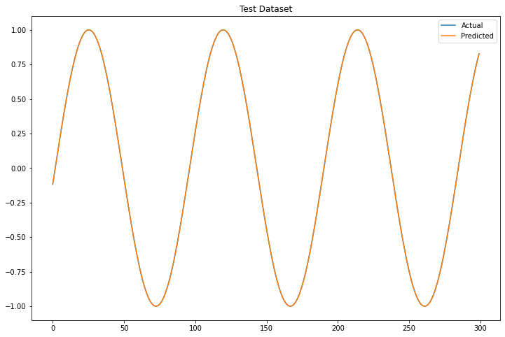
plt.title("Test Dataset")

def processData(data,lb):
    X= []
    for i in range(len(data)-lb-1):
        X.append(data[i:(i+lb),0])
    return np.array(X)

# create the x_test_dummy
cl2 =cl.copy()
pred = []
for i in range(X_test.shape[0]):
    cl2[int(X.shape[0]*0.90)+i+lb] = model.predict(X_test)[i]
    pred.extend(model.predict(X_test)[i])
    X = processData(cl2,lb)
    X_train,X_test = X[:int(X.shape[0]*0.90)],X[int(X.shape[0]*0.90):]
    X_test = X_test.reshape((X_test.shape[0],X_test.shape[1],1))


Xt = model.predict(X_test)
plt.figure(figsize=(12,8))
plt.plot(scl.inverse_transform(y_test.reshape(-1,1)), label="Actual")
plt.plot(scl.inverse_transform(Xt), label="Predicted")
plt.legend()
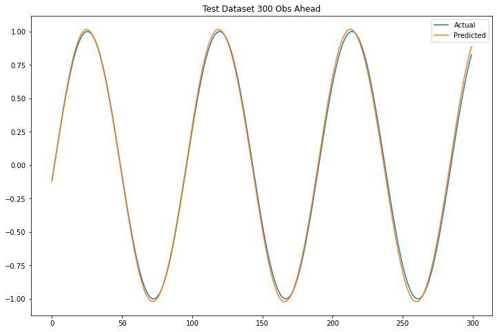
plt.title("Test Dataset 300 Obs Ahead")
 

Comments

The LSTM models captured perfectly the cosine function and has able to predict correctly 300 observations ahead.