Few words about Thompson Sampling
Thompson Sampling is an algorithm for decision problems where actions are taken in sequence balancing between exploitation which maximizes immediate performance and exploration which accumulates new information that may improve future performance. There is always a trade-off between exploration and exploitation in all Multi-armed bandit problems.
Currently, Thompson Sampling has increased its popularity since is widely used in on-line campaigns like Facebook, Youtube and Web Campaigns where many variants are served at the beginning, and as time passes, the algorithm gives more weight to the strong variants.
Conjugate Prior
In Bayesian probability theory, if the posterior distributions p(θ | x) are in the same probability distribution family as the prior probability distribution p(θ), the prior and posterior are then called conjugate distributions, and the prior is called a conjugate prior for the likelihood function p(x | θ)
Let us focus on the binomial case since in digital marketing we care mostly about CTR and Conversion Rates which follow binomial distribution. According to Bayesian Theory, the conjugate prior distribution of a Binomial Distribution is Beta Distribution with Posterior hyperparameters α and β which are the successes and the failures respectively.

Notice that The exact interpretation of the parameters of a beta distribution in terms of the number of successes and failures depends on what function is used to extract a point estimate from the distribution. The mean of a beta distribution is α/(α+β), which corresponds to α successes and β failures Bayesians generally prefer to use the posterior mean rather than the posterior mode as a point estimate, justified by a quadratic loss function, and the use of α and β is more convenient mathematically, while the use of α -1 and β -1 has the advantage that a uniform Beta(1,1) prior corresponds to 0 successes and 0 failures. The same issues apply to the Dirichlet distribution.
Thompson Sampling Algorithm
In practice, we want to maximize the expected number of rewards (i.e. clicks, conversions) given the actions (i.e. variants) and the current context. Conceptually, this means that at the beginning we serve the variants randomly and then we re-adjust our strategy (i.e. the distribution of the variants) based on the results.
The question is how do we get the weights for every state and the answer is with Monte Carlo Simulation. We assume the variants follow the Binomial distribution and according to Bayesian theory, their Conjugate prior distribution follows the Beta distribution with hyperparameters α = responses+1 and β = no responses + 1.
Let’s give an example of three variants:
- Variant 1: N=1000, responses=100 (i.e RR=10%). The conjugate prior will be Beta(a=101, b=901)
- Variant 2: N=1000, responses=110 (i.e RR=11%). The conjugate prior will be Beta(a=111, b=891)
- Variant 3: N=100, responses=10 (i.e RR=10%). The conjugate prior will be Beta(a=11, b=91)


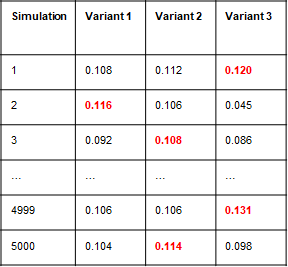
Every time we should serve the variant with the highest RR. This is done by Monte Carlo Simulation. In the example above, we sample 5000 observations of each beta distribution by picking each time the variant with the highest value. The weights we got were:
- 14% Variant 1
- 45% Variant 2
- 41% Variant 3.
Once we adjust the weights and we get new results, we follow the same approach again.
Thompson Sampling in R
It is quite easy to apply the Thompson Sampling in R. We will work with the three variants of our example above. Notice that the variant 3 has fewer impressions than the other two that is why is less steep as a distribution.
# vector of impressions per variant
b_Sent<-c(1000, 1000, 100)

# vector of responses per variant
b_Reward<-c(100, 110, 10)
msgs<-length(b_Sent)

# number of simulations
N<-5000

# simulation of Beta distributions (success+1, failures+1)
B<-matrix(rbeta(N*msgs, b_Reward+1, (b_Sent-b_Reward)+1),N, byrow = TRUE)

# Take the percentage where each variant
# was observed with the highest rate rate
P<-table(factor(max.col(B), levels=1:ncol(B)))/dim(B)[1]
P
and we get:
> P

     1      2      3
0.1368 0.4496 0.4136
Notice that since we are dealing with a Monte Carlo Simulation, if you do not set a random seed you will get slightly different results each time.
Thompson Sampling in Action
Above we showed what would be the weights the suggested weights based on the observed results of the three variants. Let’s provide an example where we are dealing with 4 Variants where we know their ground truth probability and let’s see how the Thompson Sampling will adjust the weights in every step.
Let’s assume that the ground truth conversion rates of the 4 variants are:
- Variant 1: 10%
- Variant 2: 11%
- Variant 3: 12%
- Variant 4: 13%
Our strategy is to update the weights in every 1000 impressions and let’s assume that the total sample size is 10000 (i.e. we will update the weights ten times).
output<-{}
b_Probs<-c(0.10,0.11,0.12, 0.13)
b_Sent<-rep(0, length(b_Probs))
b_Reward<-rep(0, length(b_Probs))

batch_size<-1000
N<-10000
steps<-floor(N/batch_size)
msgs<-length(b_Probs)

for (i in 1:steps) {
  B<-matrix(rbeta(batch_size*msgs, b_Reward+1, (b_Sent-b_Reward)+1),1000, byrow = TRUE)
  P<-table(factor(max.col(B), levels=1:ncol(B)))/dim(B)[1]
  # tmp are the weights for each time step
  tmp<-round(P*batch_size,0)

  # Update the Rewards
  b_Reward<-b_Reward+rbinom(rep(1,msgs), size=tmp, prob = b_Probs)

  #Update the Sent
  b_Sent<-b_Sent+tmp

  #print(P)
  output<-rbind(output, t(matrix(P)))
}

# the weights of every step
output
And we get:
> output
       [,1]  [,2]  [,3]  [,4]
 [1,] 0.239 0.259 0.245 0.257
 [2,] 0.002 0.349 0.609 0.040
 [3,] 0.003 0.329 0.533 0.135
 [4,] 0.001 0.078 0.386 0.535
 [5,] 0.001 0.016 0.065 0.918
 [6,] 0.002 0.016 0.054 0.928
 [7,] 0.002 0.095 0.154 0.749
 [8,] 0.003 0.087 0.067 0.843
 [9,] 0.001 0.059 0.069 0.871
[10,] 0.006 0.058 0.116 0.820
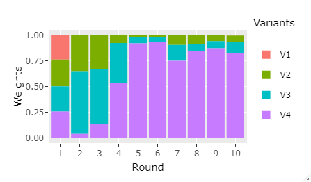
As we can see, even from the 5th step the algorithm started to assign more weight to the variant 4 and almost nothing to the variant 1 and variant 2.
Let’s see graphically how the Weights evolve across time.
library(tidyverse)

df<-as.data.frame(output)%>%mutate(Round=as.factor(row_number()))
my_plot<-df%>%gather(Variants, Weights, -Round)%>%
          ggplot(aes(x=Round, y=Weights, fill=Variants))+geom_bar(stat="identity")

my_plot

Discussion
There exist other Multi-Armed Bandit algorithms like the ε-greedy, the greedy the UCB etc. There are also contextual multi-armed bandits. In practice, there are some issues with the multi-armed bandits. Let’s mention some:
- The CTR/CR can change across days as well as the preference of the variants(seasonality effect, day of week effect, fatigue of the campaign etc)
- By changing the weights of the variants it affects the CTR/CR mainly because:
- Due to the cookies, it affects the distribution of the new and the repeated users
- The results are skewed due to the late conversions
Finally, if we provided an example of how to implement the Thompson Sampling in Python.


3 thoughts on “Multi-Armed Bandit with Thompson Sampling”
This is a fantastic and very useful post. Two comments:
1) In the post on r-bloggers.com, there are some formatting issues, for example:
The mean of a beta distribution is \(\displaystyle {\frac {\alpha }{\alpha +\beta }}\),}{\frac {\alpha }{\alpha +\beta }}, which corresponds to {\displaystyle \alpha }\alpha successes and {\displaystyle \beta }\beta failures, while the mode is {\displaystyle {\frac {\alpha -1}{\alpha +\beta -2}},}{\frac {\alpha -1}{\alpha +\beta -2}}, which corresponds to {\displaystyle \alpha -1}\alpha -1 successes and {\displaystyle \beta -1}\beta -1 failures.
2) This post solves a different problem from what is usually addressed in Multi-Armed Bandits, and that difference is not made explict in the post. Most posts on Multi-Armed Bandits assume that the choice of the next variant to show is chosen in real time, so that the selection of which arm to pull is made for each individual pull. In contrast, this post assumes that there is a manual process for assigning the percentage of pulls to assign to each arm for a set of pulls in the future – and that these percentages will be updated manually by the user from time-to-time.
I was looking for a solution to the problem this post solves and it took me a very long time to find it. So, I would suggest adding some text to clarify that difference, so that people who are looking for this solution can find it more easily.
Hi Mark,
Thanks for reaching out. We are not responsible for the formatting issues on r-bloggers.
The approach that we describe is a multi-armed bandit in batches. There is no manual work, you can automate the process