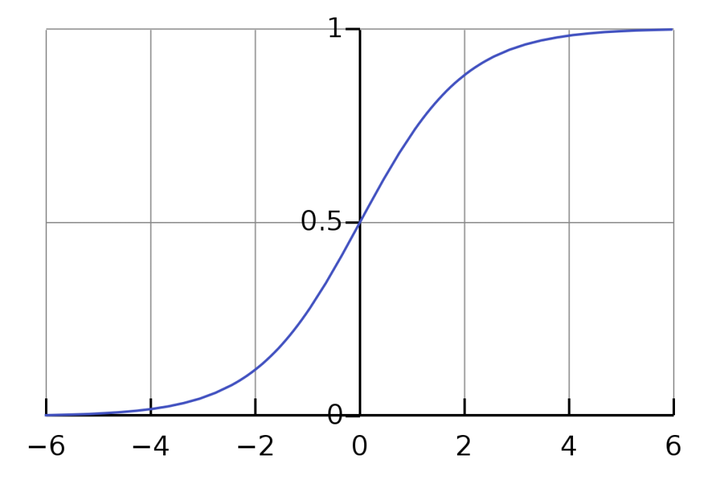
We will provide an example of how you can run a logistic regression in R when the data are grouped. Let’s provide some random sample data of 200 observations.
library(tidyverse)
set.seed(5)

df<-tibble(Gender = as.factor(sample(c("m","f"), 200, replace = TRUE, prob=c(0.6,0.4))),
           Age_Group = as.factor(sample(c("[<30]","[30-65]", "[65+]"), 200, replace = TRUE, prob=c(0.3,0.6,0.1))),
           Response = rbinom(200, 1, prob = 0.2))

df
Output:
# A tibble: 200 x 3
   Gender Age_Group Response
   <fct>  <fct>        <int>
 1 f      [65+]            0
 2 m      [30-65]          0
 3 m      [65+]            0
 4 m      [30-65]          0
 5 m      [<30]            0
 6 m      [<30]            0
 7 m      [30-65]          0
 8 m      [30-65]          0
 9 f      [<30]            1
10 f      [<30]            0
# ... with 190 more rows
Logistic Regression on Non-Aggregate Data
The logistic regression model is the following:
model1<-glm(Response ~ Gender+Age_Group, data = df, family = binomial("logit"))

summary(model1)
Output:
Call:
glm(formula = Response ~ Gender + Age_Group, family = binomial("logit"),
    data = df)

Deviance Residuals:
    Min       1Q   Median       3Q      Max
-0.7039  -0.6246  -0.6094  -0.5677   1.9754

Coefficients:
                 Estimate Std. Error z value Pr(>|z|)
(Intercept)      -1.32296    0.40899  -3.235  0.00122 **
Genderm           0.05402    0.38041   0.142  0.88707
Age_Group[30-65] -0.26642    0.42010  -0.634  0.52596
Age_Group[65+]   -0.47482    0.59460  -0.799  0.42455
---
Signif. codes:  0 ‘***’ 0.001 ‘**’ 0.01 ‘*’ 0.05 ‘.’ 0.1 ‘ ’ 1

(Dispersion parameter for binomial family taken to be 1)

    Null deviance: 188.56  on 199  degrees of freedom
Residual deviance: 187.83  on 196  degrees of freedom
AIC: 195.83

Number of Fisher Scoring iterations: 4
Logistic Regression on Aggregate Data
Assume now that you have received the data in an aggregated form and you were asked to run logistic regression. First, we need to generate the aggregate data.
df_agg<-df%>%group_by(Gender, Age_Group)%>%summarise(Impressions=n(), Responses=sum(Response))%>%
  ungroup()%>%mutate(RR=Responses/Impressions)

df_agg
Output:
# A tibble: 6 x 5
  Gender Age_Group Impressions Responses    RR
  <fct>  <fct>           <int>     <int> <dbl>
1 f      [<30]              21         6 0.286
2 f      [30-65]            49         7 0.143
3 f      [65+]               9         1 0.111
4 m      [<30]              30         5 0.167
5 m      [30-65]            66        13 0.197
6 m      [65+]              25         4 0.16
Below we will represent three different solutions.
Logistic Regression with Weights
m2<-glm(RR ~ Gender+Age_Group, data=df_agg, weights = Impressions, family = binomial("logit"))
summary(m2)
Output:
Call:
glm(formula = RR ~ Gender + Age_Group, family = binomial("logit"),
    data = df_agg, weights = Impressions)

Deviance Residuals:
      1        2        3        4        5        6
 0.8160  -0.5077  -0.2754  -0.7213   0.4145   0.1553

Coefficients:
                 Estimate Std. Error z value Pr(>|z|)
(Intercept)      -1.32296    0.40899  -3.235  0.00122 **
Genderm           0.05402    0.38042   0.142  0.88707
Age_Group[30-65] -0.26642    0.42010  -0.634  0.52596
Age_Group[65+]   -0.47482    0.59460  -0.799  0.42455
---
Signif. codes:  0 ‘***’ 0.001 ‘**’ 0.01 ‘*’ 0.05 ‘.’ 0.1 ‘ ’ 1

(Dispersion parameter for binomial family taken to be 1)

    Null deviance: 2.4477  on 5  degrees of freedom
Residual deviance: 1.7157  on 2  degrees of freedom
AIC: 29.167

Number of Fisher Scoring iterations: 4
Logistic Regression with cbind
We will need to create another column called of the No Responses and then we can use the cbind:
df_agg$No_Responses <- df_agg$Impressions- df_agg$Responses

m3<-glm(cbind(Responses, No_Responses) ~ Gender+Age_Group, data=df_agg, family = binomial("logit"))

summary(m3)
Output:
Call:
glm(formula = cbind(Responses, No_Responses) ~ Gender + Age_Group,
    family = binomial("logit"), data = df_agg)

Deviance Residuals:
      1        2        3        4        5        6
 0.8160  -0.5077  -0.2754  -0.7213   0.4145   0.1553

Coefficients:
                 Estimate Std. Error z value Pr(>|z|)
(Intercept)      -1.32296    0.40899  -3.235  0.00122 **
Genderm           0.05402    0.38042   0.142  0.88707
Age_Group[30-65] -0.26642    0.42010  -0.634  0.52596
Age_Group[65+]   -0.47482    0.59460  -0.799  0.42455
---
Signif. codes:  0 ‘***’ 0.001 ‘**’ 0.01 ‘*’ 0.05 ‘.’ 0.1 ‘ ’ 1

(Dispersion parameter for binomial family taken to be 1)

    Null deviance: 2.4477  on 5  degrees of freedom
Residual deviance: 1.7157  on 2  degrees of freedom
AIC: 29.167

Number of Fisher Scoring iterations: 4
Expand the Aggregate Data
Finally, another approach will be to transform the aggregate data to the binary form of 0 and 1. Let’s do it:
df2 <- df_agg %>% mutate(New_Response = map2(Responses, Impressions,
                            ~ c(rep(1, .x),
                                rep(0, .y - .x))))%>%unnest(cols = c(New_Response))

df2
Output:
# A tibble: 200 x 7
   Gender Age_Group Impressions Responses    RR No_Responses New_Response
   <fct>  <fct>           <int>     <int> <dbl>        <int>        <dbl>
 1 f      [<30]              21         6 0.286           15            1
 2 f      [<30]              21         6 0.286           15            1
 3 f      [<30]              21         6 0.286           15            1
 4 f      [<30]              21         6 0.286           15            1
 5 f      [<30]              21         6 0.286           15            1
 6 f      [<30]              21         6 0.286           15            1
 7 f      [<30]              21         6 0.286           15            0
 8 f      [<30]              21         6 0.286           15            0
 9 f      [<30]              21         6 0.286           15            0
10 f      [<30]              21         6 0.286           15            0
# ... with 190 more rows
And now we can run similarly with what we did at the beginning.
model4<-glm(New_Response ~ Gender+Age_Group, data = df2, family = binomial("logit"))
summary(model4)
Output:
Call:
glm(formula = New_Response ~ Gender + Age_Group, family = binomial("logit"),
    data = df2)

Deviance Residuals:
    Min       1Q   Median       3Q      Max
-0.7039  -0.6246  -0.6094  -0.5677   1.9754

Coefficients:
                 Estimate Std. Error z value Pr(>|z|)
(Intercept)      -1.32296    0.40899  -3.235  0.00122 **
Genderm           0.05402    0.38041   0.142  0.88707
Age_Group[30-65] -0.26642    0.42010  -0.634  0.52596
Age_Group[65+]   -0.47482    0.59460  -0.799  0.42455
---
Signif. codes:  0 ‘***’ 0.001 ‘**’ 0.01 ‘*’ 0.05 ‘.’ 0.1 ‘ ’ 1

(Dispersion parameter for binomial family taken to be 1)

    Null deviance: 188.56  on 199  degrees of freedom
Residual deviance: 187.83  on 196  degrees of freedom
AIC: 195.83

Number of Fisher Scoring iterations: 4
The Takeaway
With all 4 models, we came up with the same coefficients and p-values. However, in the aggregate form, we get different output regarding the deviance and the AIC score compared to the binary form.


