
In this tutorial, we will provide you an example of how you can build a powerful neural network model to classify images of cats and dogs using transfer learning by considering as base model a pre-trained model trained on ImageNet and then we will train additional new layers for our cats and dogs classification model.
The Data
We will work with a sample of 600 images from the Dogs vs Cats dataset, which was used for a 2013 Kaggle competition.
import tensorflow as tf
from tensorflow.keras.models import  Sequential, Model, load_model
from tensorflow.keras.layers import Input, Conv2D, MaxPooling2D, Dense, Flatten, Dropout
import numpy as np
import os
import pandas as pd
from sklearn.metrics import confusion_matrix
import matplotlib.pyplot as plt
%matplotlib inline
import seaborn as sns


# load the train validation and test datasets
images_train = np.load('data/images_train.npy') / 255.
images_valid = np.load('data/images_valid.npy') / 255.
images_test = np.load('data/images_test.npy') / 255.

labels_train = np.load('data/labels_train.npy')
labels_valid = np.load('data/labels_valid.npy')
labels_test = np.load('data/labels_test.npy')
Output:
600 training data examples
300 validation data examples
300 test data examples
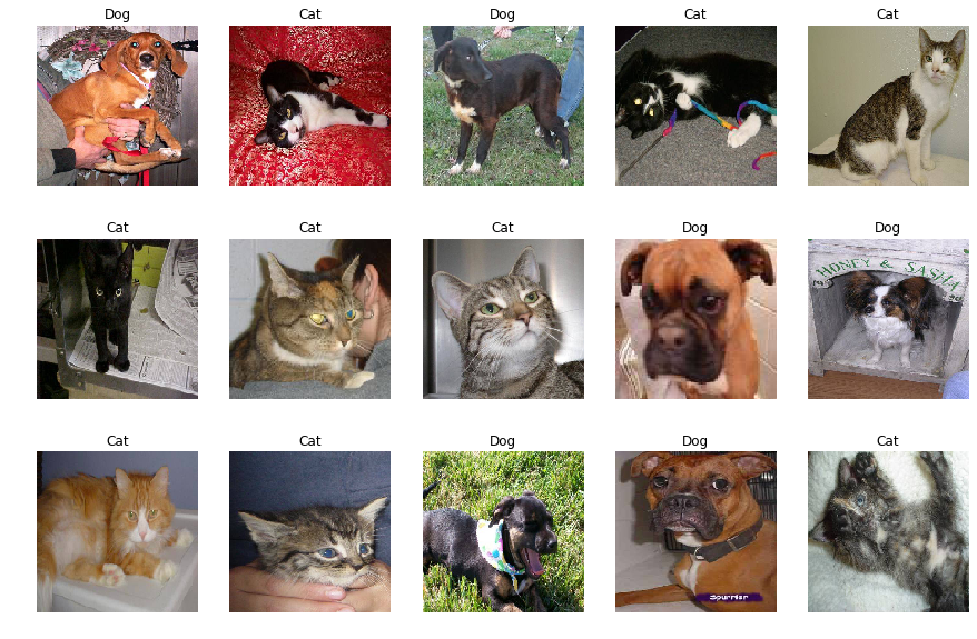
# Display a few images and labels

class_names = np.array(['Dog', 'Cat'])

plt.figure(figsize=(15,10))
inx = np.random.choice(images_train.shape[0], 15, replace=False)
for n, i in enumerate(inx):
    ax = plt.subplot(3,5,n+1)
    plt.imshow(images_train[i])
    plt.title(class_names[labels_train[i]])
    plt.axis('off')
Load the Base Model
Our base model will be the pre-trained MobileNet V2 model.
base_model = tf.keras.applications.MobileNetV2()
Use the pre-trained model as a feature extractor
We will remove the final layer of the network and replace it with new, untrained classifier layers for our task. We will create a new model that has the same input tensor as the MobileNetV2 model, and uses the output tensor from the layer with name global_average_pooling2d_6 as the model output.
feature_extractor = Model(inputs=base_model.input,
                          outputs=base_model.get_layer('global_average_pooling2d_6').output)
Build the Final Model
The final model will:
- Start with the feature extractor model that we built above.
- We will add a dense layer with 32 units and ReLU activation function.
- Then a drop out layer (50%).
- The final layer is a Dense Layer of a 1 neuron and the the activation function is the sigmoid.
final_model = Sequential([
                    feature_extractor,
                    Dense(32, activation='relu'),
                    Dropout(0.5),
                    Dense(1, activation='sigmoid')
                    ])

final_model.summary()
Output:
Model: "sequential_1"
_________________________________________________________________
Layer (type)                 Output Shape              Param #
=================================================================
model_1 (Model)              (None, 1280)              2257984
_________________________________________________________________
dense_2 (Dense)              (None, 32)                40992
_________________________________________________________________
dropout_1 (Dropout)          (None, 32)                0
_________________________________________________________________
dense_3 (Dense)              (None, 1)                 33
=================================================================
Total params: 2,299,009
Trainable params: 2,264,897
Non-trainable params: 34,112
Freeze the weights of the pre-trained model
We will freeze the weights of the pre-trained feature extractor, so that only the weights of the new layers we have added will change during the training. Finally, we will compile the final model.
final_model.layers[0].trainable = False

final_model.compile(optimizer=tf.keras.optimizers.RMSprop(0.001),
              loss = 'binary_crossentropy',
              metrics = ['acc'])

final_model.summary()
Output:
Model: "sequential_1"
_________________________________________________________________
Layer (type)                 Output Shape              Param #
=================================================================
model_1 (Model)              (None, 1280)              2257984
_________________________________________________________________
dense_2 (Dense)              (None, 32)                40992
_________________________________________________________________
dropout_1 (Dropout)          (None, 32)                0
_________________________________________________________________
dense_3 (Dense)              (None, 1)                 33
=================================================================
Total params: 2,299,009
Trainable params: 41,025
Non-trainable params: 2,257,984
Notice how the Non-trainable params changed from 34,112 to 2,257,984
Train and Evaluate the Model
We will train the model using EarlyStopping.
earlystopping = tf.keras.callbacks.EarlyStopping(patience=2)
history_frozen_new_model = final_model.fit(images_train, labels_train, epochs=10, batch_size=32,
                                                validation_data=(images_valid, labels_valid),
                                                callbacks=[earlystopping])
Output:
Train on 600 samples, validate on 300 samples
Epoch 1/10
600/600 [==============================] - 164s 273ms/sample - loss: 0.5017 - acc: 0.7517 - val_loss: 0.3234 - val_acc: 0.8467
Epoch 2/10
600/600 [==============================] - 155s 259ms/sample - loss: 0.3085 - acc: 0.8700 - val_loss: 0.2127 - val_acc: 0.8967
Epoch 3/10
600/600 [==============================] - 154s 256ms/sample - loss: 0.2082 - acc: 0.9083 - val_loss: 0.1998 - val_acc: 0.9167
Epoch 4/10
600/600 [==============================] - 153s 255ms/sample - loss: 0.2168 - acc: 0.9167 - val_loss: 0.1707 - val_acc: 0.9467
Epoch 5/10
600/600 [==============================] - 149s 249ms/sample - loss: 0.1765 - acc: 0.9367 - val_loss: 0.1550 - val_acc: 0.9500
Epoch 6/10
600/600 [==============================] - 152s 253ms/sample - loss: 0.2027 - acc: 0.9183 - val_loss: 0.1293 - val_acc: 0.9567
Epoch 7/10
600/600 [==============================] - 156s 260ms/sample - loss: 0.1557 - acc: 0.9350 - val_loss: 0.1828 - val_acc: 0.9300
Epoch 8/10
600/600 [==============================] - 155s 258ms/sample - loss: 0.1088 - acc: 0.9633 - val_loss: 0.1298 - val_acc: 0.9600
Plot the learning curves
plt.figure(figsize=(15,5))
plt.subplot(121)
try:
    plt.plot(history_frozen_new_model.history['accuracy'])
    plt.plot(history_frozen_new_model.history['val_accuracy'])
except KeyError:
    plt.plot(history_frozen_new_model.history['acc'])
    plt.plot(history_frozen_new_model.history['val_acc'])
plt.title('Accuracy vs. epochs')
plt.ylabel('Accuracy')
plt.xlabel('Epoch')
plt.legend(['Training', 'Validation'], loc='lower right')

plt.subplot(122)
plt.plot(history_frozen_new_model.history['loss'])
plt.plot(history_frozen_new_model.history['val_loss'])
plt.title('Loss vs. epochs')
plt.ylabel('Loss')
plt.xlabel('Epoch')
plt.legend(['Training', 'Validation'], loc='upper right')
plt.show()

Evaluate the new model
new_model_test_loss, new_model_test_acc = final_model.evaluate(images_test, labels_test, verbose=0)
print("Test loss: {}".format(new_model_test_loss))
print("Test accuracy: {}".format(new_model_test_acc))
Output:
Test loss: 0.10817002788186074
Test accuracy: 0.9566666483879089
We got an accuracy of 96%. Not bad!
References:
[1] Coursera Customising your models with TensorFlow 2