Portfolio Optimization in Python

We will show how you can build a diversified portfolio that satisfies specific constraints. For this tutorial, we will build a portfolio that minimizes the risk.

So the first thing to do is to get the stock prices programmatically using Python.

How to Download the Stock Prices using Python

We will work with the yfinance package where you can install it using pip install yfinance --upgrade --no-cache-dir You will need to get the symbol of the stock. You can find the mapping between NASDAQ stocks and symbols in this csv file.

For this tutorial, we will assume that we are dealing with the following 10 stocks and we try to minimize the portfolio risk.

• Google with Symbol GOOGL
• Tesla with Symbol TSLA
• Facebook with Symbol FB
• Amazon with Symbol AMZN
• Apple with Symbol AAPL
• Microsoft with Symbol MSFT
• Vodafone with Symbol VOD
• Adobe with Symbol ADBE
• NVIDIA with Symbol NVDA
• Salesforce with Symbol CRM

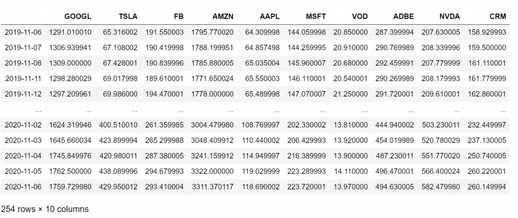
We will download the close prices for the last year.

import pandas as pd
import numpy as np
import yfinance as yf
from scipy.optimize import minimize
import matplotlib.pyplot as plt
%matplotlib inline  



symbols = ['GOOGL', 'TSLA', 'FB', 'AMZN', 'AAPL', 'MSFT', 'VOD',  'ADBE', 'NVDA', 'CRM' ]

all_stocks = pd.DataFrame()

for symbol in symbols:
    tmp_close = yf.download(symbol, 
                      start='2019-11-07', 
                      end='2020-11-07', 
                      progress=False)['Close']
    all_stocks = pd.concat([all_stocks, tmp_close], axis=1)

all_stocks.columns=symbols
all_stocks
 

---

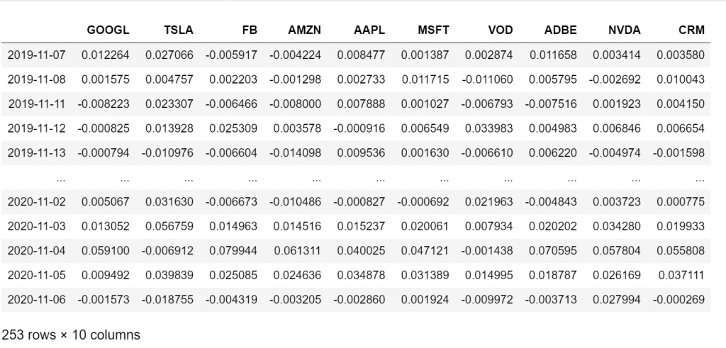
Get the Log Returns

We will use the log returns or continuously compounded return. Let’s calculate them in Python.

returns = np.log(all_stocks/all_stocks.shift(1)).dropna(how="any")
returns
 

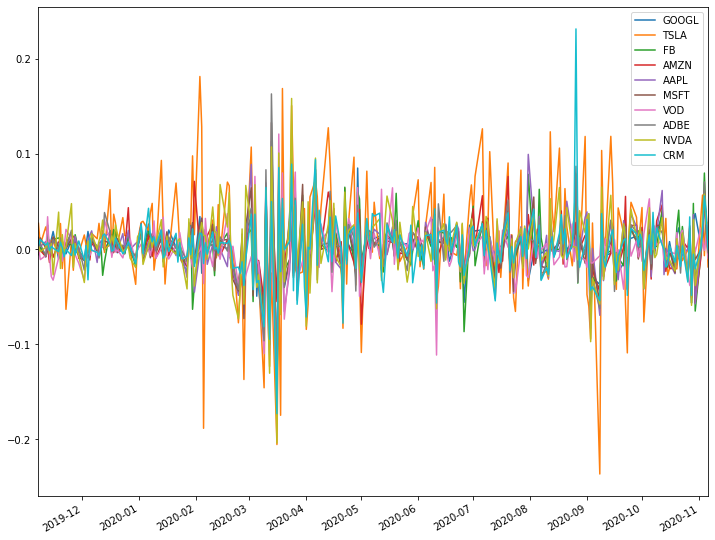
returns.plot(figsize=(12,10))
 

---

Get the Mean Returns

We can get the mean returns of every stock as well as the average of all of them.

# mean daily returns per stock 
returns.mean()
 

GOOGL    0.001224
TSLA     0.007448
FB       0.001685
AMZN     0.002419
AAPL     0.002422
MSFT     0.001740
VOD     -0.001583
ADBE     0.002146
NVDA     0.004077
CRM      0.001948
dtype: float64

# mean daily returns of all stocks
returns.mean().mean()

0.0023526909011353354
 

---

Minimize the Risk of the Portfolio

Our goal is to construct a portfolio from those 10 stocks with the following constraints:

• The Expected daily return is higher than the average of all of them, i.e. greater than 0.003
• There is no short selling, i.e. we only buy stocks, so the sum of the weights of all stocks will ad up to 1
• Every stock can get a weight from 0 to 1, i.e. we can even build a portfolio of only one stock, or we can exclude some stocks.

Finally, our objective is to minimize the variance (i.e. risk) of the portfolio. You can find a nice explanation on this blog of how you can calculate the variance of the portfolio using matrix operations.

We will work with the scipy library:

# the objective function is to minimize the portfolio risk
def objective(weights): 
    weights = np.array(weights)
    return weights.dot(returns.cov()).dot(weights.T)



# The constraints
cons = (# The weights must sum up to one.
        {"type":"eq", "fun": lambda x: np.sum(x)-1}, 
        # This constraints says that the inequalities (ineq) must be non-negative.
        # The expected daily return of our portfolio and we want to be at greater than 0.003
        {"type": "ineq", "fun": lambda x: np.sum(returns.mean()*x)-0.003}) 


# Every stock can get any weight from 0 to 1
bounds = tuple((0,1) for x in range(returns.shape[1])) 

# Initialize the weights with an even split
# In out case each stock will have 10% at the beginning
guess = [1./returns.shape[1] for x in range(returns.shape[1])]


optimized_results = minimize(objective, guess, method = "SLSQP", bounds=bounds, constraints=cons)
optimized_results

Output:

     fun: 0.0007596800848097395
     jac: array([0.00113375, 0.00236566, 0.00127447, 0.0010218 , 0.00137465,
       0.00137397, 0.00097843, 0.00144561, 0.00174113, 0.0014457 ])
 message: 'Optimization terminated successfully.'
    nfev: 24
     nit: 2
    njev: 2
  status: 0
 success: True
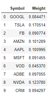
       x: array([0.08447057, 0.17051382, 0.09077398, 0.10128927, 0.10099533,
       0.09145521, 0.04536969, 0.09705495, 0.12378042, 0.09429676])

The optimum weights are the array x and we can retrieve them as follows:

optimized_results.x
 

Output:

array([ 8.44705689, 17.05138189,  9.07739784, 10.12892656, 10.09953316,
        9.14552072,  4.53696906,  9.70549545, 12.37804203,  9.42967639])

We can check that the weights sum up to 1:

# we get 1
np.sum(optimized_results.x)
 

And we can see that the expected return of the portfolio is

np.sum(returns.mean()*optimized_results.x)
 

Output:

0.002999999997028756

Which is almost 0.003 (some rounding errors) which was our requirement.

Final Weights

So let’s report the optimized weights nicely.

pd.DataFrame(list(zip(symbols, optimized_results.x)), columns=['Symbol', 'Weight'])