Hierarchical Clustering in Python

We have provided an example of K-means clustering and now we will provide an example of Hierarchical Clustering. We will work with the famous Iris Dataset.

import pandas as pd
import numpy as np
import matplotlib.pyplot as plt
import seaborn as sns
%matplotlib inline 

from sklearn import datasets
iris = datasets.load_iris()


df=pd.DataFrame(iris['data'])
print(df.head())
 

     0    1    2    3
0  5.1  3.5  1.4  0.2
1  4.9  3.0  1.4  0.2
2  4.7  3.2  1.3  0.2
3  4.6  3.1  1.5  0.2
4  5.0  3.6  1.4  0.2

Let’s see the number of targets that the Iris dataset has and their frequency:

np.unique(iris.target,return_counts=True)
 

(array([0, 1, 2]), array([50, 50, 50], dtype=int64))

As we can see there are three targets of 50 observations each. If we want to see the names of the target:

iris.target_names

array(['setosa', 'versicolor', 'virginica'], dtype='<U10')

---

Data Preparation for Cluster Analysis

When we apply Cluster Analysis we need to scale our data. There are many different approaches like standardizing or normalizing the values etc. Also, we can whiten the values which is a process of rescaling data to a standard deviation of 1:

\(x_{new} = x/std\_dev(x)\)

Let’s scaled the iris dataset.

# Import the whiten function
from scipy.cluster.vq import whiten
scaled_data = whiten(df.to_numpy())
 

Let’s check if the variance of every feature is close to 1 now:

pd.DataFrame(scaled_data).describe()
 

	0	1	2	3
count	150.000000	150.000000	150.000000	150.000000
mean	7.080243	7.037882	2.135951	1.578709
std	1.003350	1.003350	1.003350	1.003350
min	5.210218	4.603935	0.568374	0.131632
25%	6.179561	6.445509	0.909399	0.394897
50%	7.027736	6.905903	2.472428	1.711218
75%	7.754744	7.596493	2.898709	2.369379
max	9.572262	10.128658	3.921782	3.290805

---

Creat the Distance Matrix based on linkage

Look at the documentation of the `linkage` function to see the available methods and metrics.

# Import the fcluster and linkage functions
from scipy.cluster.hierarchy import fcluster, linkage

# Use the linkage() function
distance_matrix = linkage(scaled_data, method = 'ward', metric = 'euclidean')
 

---

How many Clusters – Introduction to dendrograms

Dendrograms help in showing progressions as clusters are merged. It is a branching diagram that demonstrates how each cluster is composed by branching out into its child nodes.

# Import the dendrogram function
from scipy.cluster.hierarchy import dendrogram

# Create a dendrogram
dn = dendrogram(distance_matrix)

# Display the dendogram
plt.show()
 

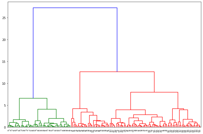
From the dendrogram we can realize that a good candidate for the number of Clusters is 3 and that 2 clusters are closer (the red ones) compared to the green one.

---

Run the Hierarchical Clustering

# Assign cluster labels
df['cluster_labels'] = fcluster(distance_matrix, 3, criterion='maxclust')
 

Notice that we can define clusters based on the linkage distance by changing the criterion to distance in the fcluster function!

---

Hierarchical vs Actual for n_clusters=3

df['target'] = iris.target

fig, axes = plt.subplots(1, 2, figsize=(16,8))
axes[0].scatter(df[0], df[1], c=df['target'])
axes[1].scatter(df[0], df[1], c=df['cluster_labels'], cmap=plt.cm.Set1)
axes[0].set_title('Actual', fontsize=18)
axes[1].set_title('Hierarchical', fontsize=18)