Detect the Changes in Timeseries Data

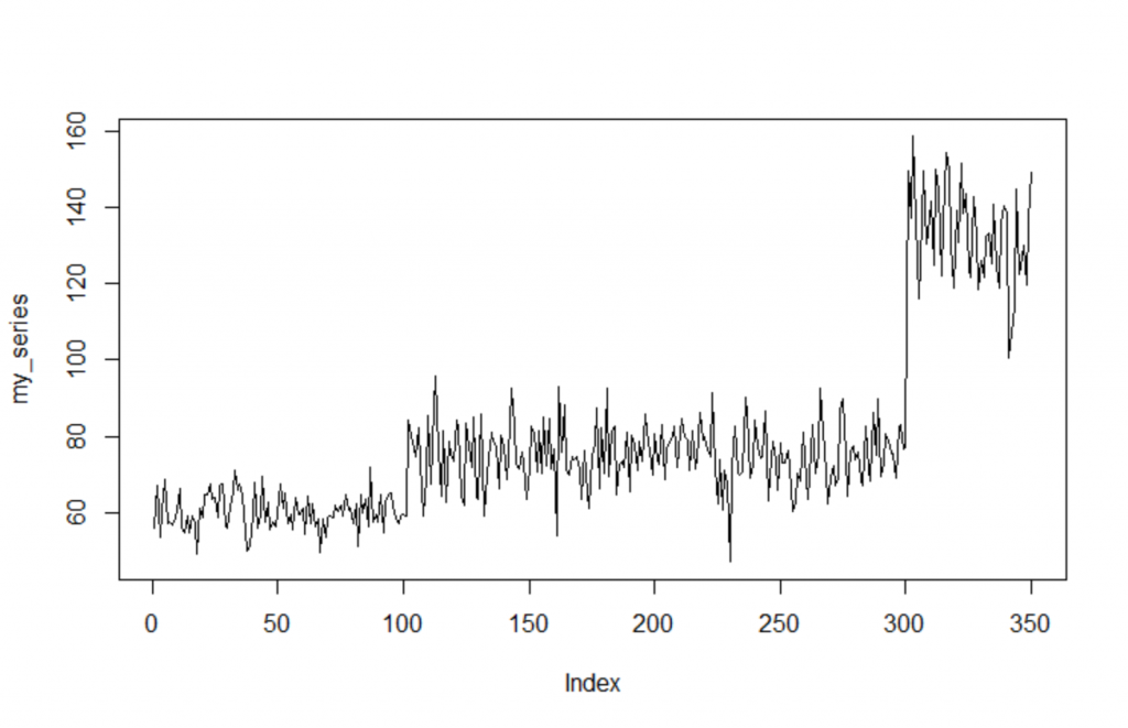
In this post, we will provide an example of how you can detect changes in the distribution across time. For example, let’s say that we monitor the heart rate of a person with the following states:

• Sleep: Normal (60,5)
• Awake: Normal (75,8)
• Exercise: Normal (135, 12)

Let’s generate this data:

set.seed(5)

sleep<-rnorm(100, 60, 5)
awake<-rnorm(200, 75, 8)
exercise<-rnorm(50, 135, 12)

my_series<-c(sleep, awake, exercise)

plot(my_series, type='l')

We can work with two different packages, the changepoint and the bcp.

Detect the Changes with the changepoint

We will try to test the changes in mean.

library(changepoint)

# change in mean
ansmean=cpt.mean(my_series, method = 'BinSeg')
plot(ansmean,cpt.col='blue')
print(ansmean)

Output:

Class 'cpt' : Changepoint Object
       ~~   : S4 class containing 14 slots with names
              cpts.full pen.value.full data.set cpttype method test.stat pen.type pen.value minseglen cpts ncpts.max param.est date version 

Created on  : Fri Mar 05 16:01:12 2021 

summary(.)  :
----------
Created Using changepoint version 2.2.2 
Changepoint type      : Change in mean 
Method of analysis    : BinSeg 
Test Statistic  : Normal 
Type of penalty       : MBIC with value, 17.5738 
Minimum Segment Length : 1 
Maximum no. of cpts   : 5 
Changepoint Locations : 101 300 303 306 324 
Range of segmentations:
     [,1] [,2] [,3] [,4] [,5]
[1,]  300   NA   NA   NA   NA
[2,]  300  101   NA   NA   NA
[3,]  300  101  324   NA   NA
[4,]  300  101  324  303   NA
[5,]  300  101  324  303  306

 For penalty values: 168249.2 15057.6 1268.036 373.3306 373.3306 

As we can see, it detected 4 distributions instead of 3.

Detect the Changes with the bcp

bcp() implements the Bayesian change point analysis methods given in Wang and Emerson (2015),
of which the Barry and Hartigan (1993) product partition model for the normal errors change point
problem is a specific case.

library(bcp)

bcp.1a <- bcp(my_series)
plot(bcp.1a, main="Univariate Change Point Example")
legacyplot(bcp.1a)
 

As we can see, it returns the posterior Mean as well as the probability of a change at that particular step. We can set a threshold like 30%. It correctly detected the two changes in the distributions at the right time (step=100 and step=300)