Contingency Tables in R

A common way to represent and analyze categorical data is through contingency tables. In this tutorial, we will provide some examples of how you can analyze two-way (r x c) and three-way (r x c x k) contingency tables in R.

Dataset

For this tutorial, we will work with the Wage dataset from the ISLR package. We will create another column of the Wage, which is categorical taking two values as Above and Below when the Wage is above or below media respectively. The format of the dataset is the following:

A data frame with 3000 observations on the following 11 variables.

• year: Year that wage information was recorded
• age: Age of worker
• marit1: A factor with levels 1. Never Married 2. Married 3. Widowed 4. Divorced and 5. Separated indicating marital status
• race: A factor with levels 1. White 2. Black 3. Asian and 4. Other indicating race
• education: A factor with levels 1. < HS Grad 2. HS Grad 3. Some College 4. College Grad and 5. Advanced Degree indicating education level
• region: Region of the country (mid-atlantic only)
• jobclass: A factor with levels 1. Industrial and 2. Information indicating type of job
• health: A factor with levels 1. <=Good and 2. >=Very Good indicating health level of worker
• health_ins: A factor with levels 1. Yes and 2. No indicating whether worker has health insurance
• logwage: Log of workers wage
• wage: Workers raw wage

Two-Way Tables

Two-way tables involve two categorical variables, X with r categories and Y with c. Therefore, there are r times c possible combinations. Sometimes, both X and Y will be response variables, in which case it makes sense to talk about their joint distribution. On other occasions, Y will be the response variable and X will be the explanatory variable. In this case, it does not make sense to talk about the joint distribution of X and Y. Instead, we focus on the conditional distribution of Y given X.

Let’s start analyzing the data. At the beginning we can see the relationship between wage_cat and Jobclass.

library(ISLR)
library(tidyverse)
library(Rfast)
library(MASS)

# create the wage_cat variable which takes two values
# such as Above if the wage is above median and Below if
# the wage is below median
Wage$wage_cat<-as.factor(ifelse(Wage$wage>median(Wage$wage),"Above","Below"))



# Examine the Wage vs Job Class
# you could use also the command xtabs(~jobclass+wage_cat, data=Wage)

con1<-table(Wage$jobclass,Wage$wage_cat)

con1

Output:

                
                 Above Below
  1. Industrial    629   915
  2. Information   854   602

Mosaic plots

The most proper way to represent graphically the contingency tables are the mosaic plots:

mosaicplot(con1)

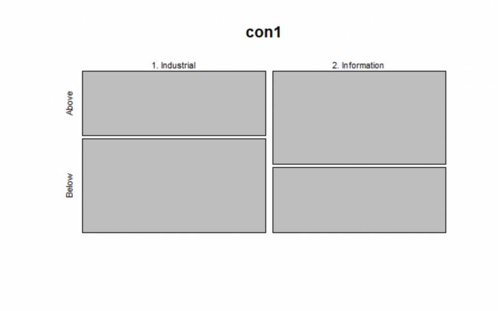
From the mosaic plot above we can easily see that in the Industrial sector the percentage of people who are below the median are more compared to those who work in the Information industry.

Proportions of the Contingency Tables

We can get the proportions of the Contingency Tables, on overall and by rows and columns. Let’s see how we can do it:

# overall
prop.table(con1)

# by row
prop.table(con1, margin = 1)

# by column
prop.table(con1, margin = 2)
 

Output:

> # overall
> prop.table(con1)
                
                     Above     Below
  1. Industrial  0.2096667 0.3050000
  2. Information 0.2846667 0.2006667
> 
> # by row
> prop.table(con1, margin = 1)
                
                     Above     Below
  1. Industrial  0.4073834 0.5926166
  2. Information 0.5865385 0.4134615
> 
> # by column
> prop.table(con1, margin = 2)
                
                     Above     Below
  1. Industrial  0.4241403 0.6031641
  2. Information 0.5758597 0.3968359

Rows and Columns Totals

We can add the rows and columns totals of the contingency tables as follows:

addmargins(con1)
 

Output:

                 Above Below  Sum
  1. Industrial    629   915 1544
  2. Information   854   602 1456
  Sum             1483  1517 3000

Statistical Tests

We can apply the following statistical tests in order to test if the relationship of these two variables is independent or not.

Chi-Square Test

We have explained the Chi-Square Test in a previous post. Let’s run it in R:

chisq.test(con1)
 

Output:

	Pearson's Chi-squared test with Yates' continuity correction

data:  con1
X-squared = 95.504, df = 1, p-value < 2.2e-16

As we can see the p-value is less than 5% thus we can reject the null hypothesis that the jobclass is independent to median wage.

Fisher’s Exact Test

When the sample size is low, we can apply the Fisher’s exact test instead of Chi-Square test.

fisher.test(con1)
 

Output:

	Fisher's Exact Test for Count Data

data:  con1
p-value < 2.2e-16
alternative hypothesis: true odds ratio is not equal to 1
95 percent confidence interval:
 0.4177850 0.5620273
sample estimates:
odds ratio 
 0.4847009 

Again, we see that we reject the null hypothesis.

Log Likelihood Ratio

Another test that we can apply is the Log Likelihood Ratio using the MASS package:

loglm( ~ 1 + 2, data = con1) 
 

Output:

Call:
loglm(formula = ~1 + 2, data = con1)

Statistics:
                      X^2 df P(> X^2)
Likelihood Ratio 96.73432  1        0
Pearson          96.21909  1        0

Again, we rejected the null hypothesis.

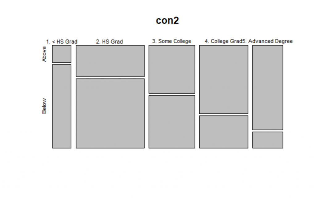
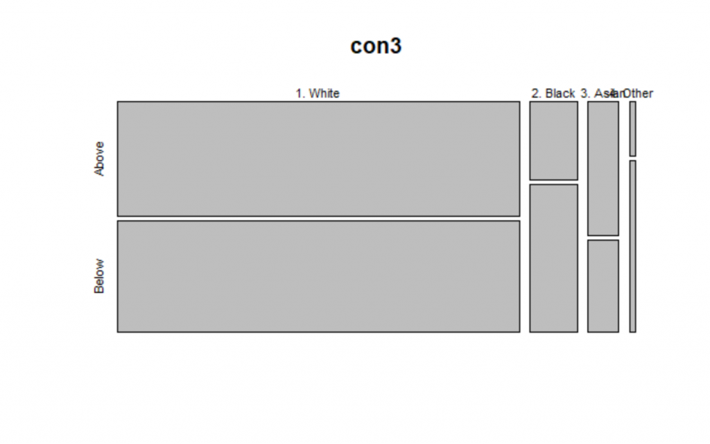
Notice that if we run the same analysis by comparing the wage median versus race and the wage median vs education, we find tha there is a statistical significance difference in both cases.

con2<-table(Wage$education,Wage$wage_cat)

con2
mosaicplot(con2)
chisq.test(con2)


con3<-table(Wage$race,Wage$wage_cat)

con3
mosaicplot(con3)
chisq.test(con3)
 

Output

Three-Way Tables

Let’s say that now we want to create contingency tables of three dimensions such as wage median, race and jobclass

con4<-xtabs(~jobclass+wage_cat+race, data=Wage)

ftable(con4)
 

Output:

                        race 1. White 2. Black 3. Asian 4. Other
jobclass       wage_cat                                         
1. Industrial  Above              558       32       36        3
               Below              767       79       50       19
2. Information Above              701       70       77        6
               Below              454      112       27        9

Let’s say that we want to change the share of the rows and columns.

con4%>%ftable(row.vars=c("race", "jobclass"))

 

Output:

                        wage_cat Above Below
race     jobclass                           
1. White 1. Industrial             558   767
         2. Information            701   454
2. Black 1. Industrial              32    79
         2. Information             70   112
3. Asian 1. Industrial              36    50
         2. Information             77    27
4. Other 1. Industrial               3    19
         2. Information              6     9

Let’s say now we want to get the probabilities by row:

con4%>%ftable(row.vars=c("race", "jobclass"))%>%prop.table(margin = 1)%>%round(2)
 

Output:

                        wage_cat Above Below
race     jobclass                           
1. White 1. Industrial            0.42  0.58
         2. Information           0.61  0.39
2. Black 1. Industrial            0.29  0.71
         2. Information           0.38  0.62
3. Asian 1. Industrial            0.42  0.58
         2. Information           0.74  0.26
4. Other 1. Industrial            0.14  0.86
         2. Information           0.40  0.60

Cochran-Mantel-Haenszel (CMH) Methods

We are dealing with a 2x2x4 table where the race has 4 levels. We want to test for conditional independence and homogeneous associations with the K conditional odds ratios in 2x2x4 table. With the CMH Methods, we can combine the sample odds ratios from the 4 partial tables into a single summary measure of partial association. In our case, we have the wage_cat (Above, Below) the jobclass (Industrial, Information) and the race (White, Black, Asian, Other). We want to investigate the association between wage_cat and jobclass while controlling for race.

The null hypothesis is that wage_cat and jobclass are conditionally independent, given the race, which means that the odds ratio of wage_cat and jobckass is 1 for all races versus at least one odds ratio is not 1.

\(H_0: θ=1\) for race is White, Black, Asian and Other.

Using the Rfast package we can get the odds ratio for each race:

#get the 4 odds ratio

for (i in 1:4) {
  
  print(odds.ratio(con4[,,i])$res[1])
}
 

Output:

odds ratio 
  0.471169 
odds ratio 
 0.6481013 
odds ratio 
 0.2524675 
odds ratio 
 0.2368421 

As we can see, the odds ratios are not close to 1, so we expect to reject the null hypothesis. Let’s run the CHM test:

#CMH Test

mantelhaen.test(con4)
 

Output:

	Mantel-Haenszel chi-squared test with continuity correction

data:  con4
Mantel-Haenszel X-squared = 104.45, df = 1, p-value < 2.2e-16
alternative hypothesis: true common odds ratio is not equal to 1
95 percent confidence interval:
 0.4003835 0.5381067
sample estimates:
common odds ratio 
        0.4641649 

As expected, we rejected the null hypothesis since the p-value is less than 5%.

Conclusion

The contingency tables is the best way to represent and analyze the relationship between categorical variables. The Cochran-Mantel-Haenszel is the proper test for 2x2xk tables and is a good approach when we are dealing with cases that have the Simpson’s Paradox.