Confidence vs Credible Intervals for Proportions

In Frequentist Statistics we communicate the Confidence Intervals where in Bayesian Statistics we communicate the Credible Intervals.

In this post we are not going to dive into formulas and theory. On contrary our goal is to give an example of how we can calculate the Confidence and the Credible Intervals using R and to see their differences.

The main difference is that according to Frequentists the Binomial distribution follows approximately the normal distribution \(N\sim(p,\frac{p(1-p)}{n})\) while according to Bayesians the conjugate prior is the beta distribution with shape parameters \(\alpha=Successes+1\) and \(\beta=Failures+1\)

Let’s consider the following example where the \(n=1000\), the \(p=20\%\) and we want to calculate the \(95\%\) Confidence and Credible Intervals.

# Probability 20%
p<-0.2
# sample size n=1000
n=1000
# alpha=5% since we want the 95% confidence and credible intervals
alpha=0.05


# 95% Confidence Interval
qnorm(c(alpha/2,(1-alpha/2)), mean=p, sd=sqrt((p*(1-p))/n))

0.1752082 0.2247918

Now we are going to calculate the Credible interval:

# 95% Credible Interval
qbeta(c(alpha/2,(1-alpha/2)), (n*p)+1, (n-n*p)+1)

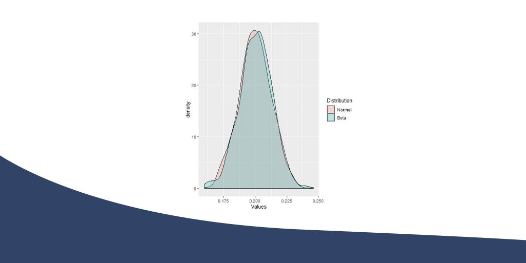
0.1763924 0.2259372

As we can see the differences are quite small. Let’s see what are the density functions of the Normal and Beta of our example.

library(ggplot2)

df1<-data.frame(Values = rnorm(1000, p, sqrt(p*(1-p)/n) ), Distribution="Normal")
df2<-data.frame(Values = rbeta(1000, (n*p)+1, (n-n*p)+1 ), Distribution="Beta")
df<-rbind(df1,df2)
ggplot(df, aes(x=Values, fill=Distribution))+geom_density(alpha=0.25)