Introduction

We will provide a walk-through tutorial of the “Data Science Pipeline” that can be used as a guide for Data Science Projects. We will consider the following phases:

1. Data Collection/Curation
2. Data Management/Representation
3. Exploratory Data Analysis
4. Hypothesis Testing and Machine Learning
5. Communication of insights attened

For this project we will consider a supervised machine learning problem, and more particularly a regression model.

The Regression models involve the following components:

• The unknown parameters are often denoted as a scalar or vector \(β\) .
• The independent variables, which are observed in data and are often denoted as a vector \(X_i\).
• The dependent variable, which is observed in data and often denoted using the scalar \(Y_i\).
  The error terms, which are not directly observed in data and are often denoted using the scalar \(e_i\).

This tutorial is based on the Python programming language and we will work with different libraries like pandas, numpy, matplotlib, scikit-learn and so on. Finally, in this tutorial, we provide references and resources in the form of hyperlinks.

Data Collection/Curation

The UC Irvine Machine Learning Repository is a Machine Learning Repository which maintains 585 data sets as a service to the machine learning community. You may view all data sets through our searchable interface. For a general overview of the Repository, please visit our About page. For information about citing data sets in publication. For our project, we chose to work with the Bike Sharing Dataset Data Set.

Bike Sharing Dataset

This dataset contains the hourly count of rental bikes between 2011 and 2012 in Capital bikeshare system with the corresponding weather and seasonal information. Our goal is to build a Machine Learning model which will be able to predict the count of rental bikes.

Data Management/Representation

The fields of our dataset are the following:

- instant: record index
- dteday : date
- season : season (1:springer, 2:summer, 3:fall, 4:winter)
- yr : year (0: 2011, 1:2012)
- mnth : month ( 1 to 12)
- hr : hour (0 to 23)
- holiday : weather day is holiday or not (extracted from http://dchr.dc.gov/page/holiday-schedule)
- weekday : day of the week
- workingday : if day is neither weekend nor holiday is 1, otherwise is 0.
+ weathersit : 
    - 1: Clear, Few clouds, Partly cloudy, Partly cloudy
    - 2: Mist + Cloudy, Mist + Broken clouds, Mist + Few clouds, Mist
    - 3: Light Snow, Light Rain + Thunderstorm + Scattered clouds, Light Rain + Scattered clouds
    - 4: Heavy Rain + Ice Pallets + Thunderstorm + Mist, Snow + Fog
- temp : Normalized temperature in Celsius. The values are divided to 41 (max)
- atemp: Normalized feeling temperature in Celsius. The values are divided to 50 (max)
- hum: Normalized humidity. The values are divided to 100 (max)
- windspeed: Normalized wind speed. The values are divided to 67 (max)
- casual: count of casual users
- registered: count of registered users
- cnt: count of total rental bikes including both casual and registered

Let’s start the analysis by loading the data.

df = pd.read_csv("hour.csv")
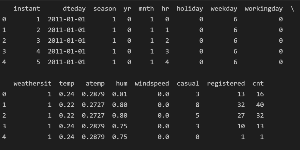
# get the first rows
df.head()

Feature Leakage

If we look carefully at our data, we will see that the addition of the casual and registered columns yield to the cnt column. This is what we call leakage and for that reason, we will remove them from our dataset. The reason for that is when we want to predict the total Bike Rentals cnt, we will have as “known” independent variables the “casual” and the “registered” which is not true, since by the time of prediction we will lack this info.

# drop the 'casual' and 'registered' columns
df.drop(['casual', 'registered'], axis=1, inplace=True)

### Remove the instant column
We will also remove the `instant` from our model since is not an explanatory variable.

Transform the Columns to the Right Data Type.

We will change the Data Type of the following columns:

• dteday: Conver it to Date
• season: Convert it to Categorical
• weekday: Convert it to Categorical
• mnth: Conver it to Categorical

# let's convert them
df['dteday'] = pd.to_datetime(df['dteday'])
df['season'] = df['season'].astype("category")
df['weekday'] = df['weekday'].astype("category")
df['mnth'] = df['mnth'].astype("category")

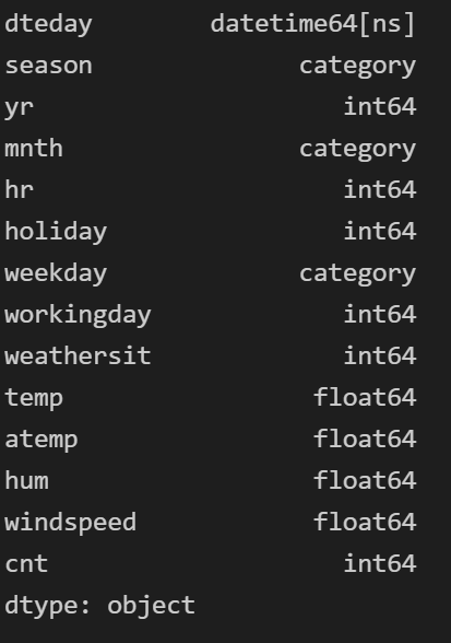
# check the data types
df.dtypes

Check for Missing Values

At this point, we will check for any missing values in our data.

df.isna().sum()

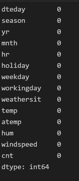
As we can see there is no missing value in any field.

Check for Duplicated Values

At this point, we will check if there are duplicated values, where as we can see below, there are no duplicated values. So, we are ok to proceed.

df.duplicated().sum()

0

Description of the Dataset

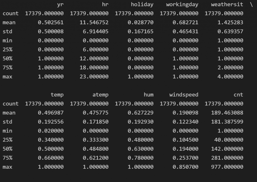
Let’s see a summary of our data fields for the continuous variables by showing the mean, std, min, max, and Q2,Q3.

df.describe()

Finally, let’s get the number of rows and columns of our dataset so far.

df.shape

(17379, 14)

Exploratory Data Analysis

At this point, we run an EDA. Let’s have a look at the Bike Rentals across time.

Time Series Plot of Hourly Rental Bikes

df.plot(x='dteday', y='cnt', figsize=(20,12), title = 'Hourly Rental Bikes')
plt.ylabel('cnt')

Distribution of the Rental Bikes

df['cnt'].plot.hist(bins=20, figsize=(12,8))

Box Plots of Bike Rentals

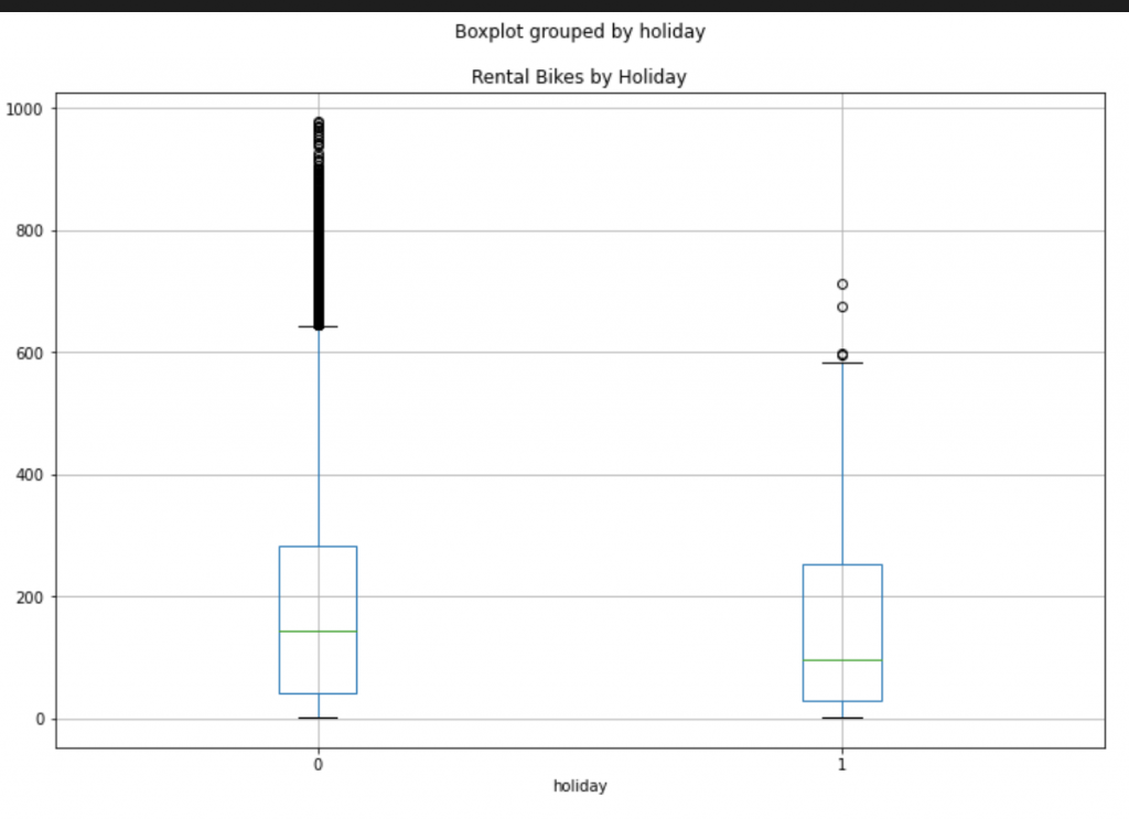
df.boxplot(by='mnth', column='cnt', figsize=(12,8))
plt.title("Rental Bikes by Month")

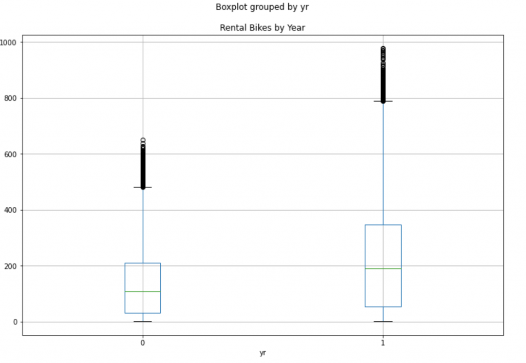
df.boxplot(by='yr', column='cnt', figsize=(12,8))
plt.title("Rental Bikes by Year")

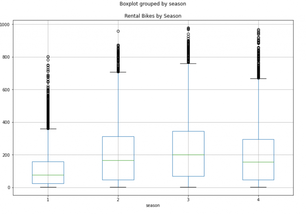
df.boxplot(by='season', column='cnt', figsize=(12,8))
plt.title("Rental Bikes by Season")

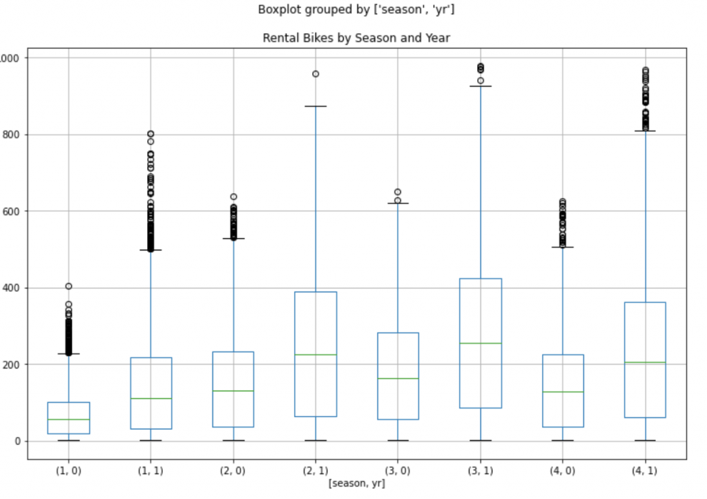
df.boxplot(by=['season','yr'], column='cnt', figsize=(12,8))
plt.title("Rental Bikes by Season and Year")

df.boxplot(by=['hr'], column='cnt', figsize=(12,8))
plt.title("Rental Bikes by Hour")

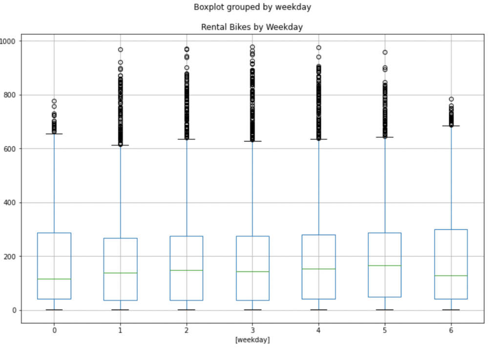
df.boxplot(by=['weekday'], column='cnt', figsize=(12,8))
plt.title("Rental Bikes by Weekday")

Correlation and Correlation Heat Map

We will return the correlation Pearson coefficient of the numeric variables.

# get the correlation

df.corr()

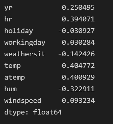
# correlation of Rental Bikes vs the rest variables
df.drop('cnt', axis=1).corrwith(df.cnt)

plt.figure(figsize=(12,8))
sns.heatmap(df.corr(), annot=True, cmap="YlGnBu")

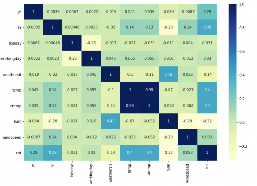
Multi-Collinearity

As expected the temp and atemp are strongly correlated causing a problem of muticollinearity and that is why we will keep only one. We will remove the temp.

df.drop('temp', axis=1, inplace=True)

# remove also the date column since we will not use it for the machine learning modelling
df.drop('dteday', axis=1, inplace=True)

Hypothesis Testing and Machine Learning

Before we start analysing our models, we will need to apply one-hot encoding to the categorical variables. We will do that by applying the get_dummies function.

One-Hot Encoding

df = pd.get_dummies(df)

Train-Test Dataset

For our analysis we split the dataset into train and test (75% -25%) so that to build the models on the train dataset and to evaluate them on the test dataset.

X_train, X_test, y_train, y_test = train_test_split(df.drop('cnt', axis=1), df.cnt, test_size=0.25, random_state=5)

Machine Learning Models

We will try different machine learning models

• Linear Regression
• Random Forest
• Gradient Boost

and we will choose the one with the lowest RMSE.

Linear Regression

from sklearn.metrics import mean_squared_error
from sklearn.linear_model import LinearRegression

reg = LinearRegression().fit(X_train, y_train)

# Get the RMSE for the train dataset
print(np.sqrt(mean_squared_error(y_train, reg.predict(X_train))))

# Get the RMSE for the test dataset
print(np.sqrt(mean_squared_error(y_test, reg.predict(X_test))))

139.63173269641877
141.72019878710364

Random Forest

from sklearn.ensemble import RandomForestRegressor

rf = RandomForestRegressor().fit(X_train, y_train)

# Get the RMSE for the train dataset
print(np.sqrt(mean_squared_error(y_train, rf.predict(X_train))))

# Get the RMSE for the test dataset
print(np.sqrt(mean_squared_error(y_test, rf.predict(X_test))))

16.301139181478824
42.60910391839956

Gradient Boost

from sklearn.ensemble import GradientBoostingRegressor

gb = GradientBoostingRegressor().fit(X_train, y_train)

# Get the RMSE for the train dataset
print(np.sqrt(mean_squared_error(y_train, gb.predict(X_train))))

# Get the RMSE for the test dataset
print(np.sqrt(mean_squared_error(y_test, gb.predict(X_test))))

69.83046975214577
69.94424353189753

Choose the Best Model

Based on the RMSE on both train and test dataset, the best model is the Random Forest.

Statistical Analysis

Based on the statistical analysis and the Gini, we will define the most important variables of the Random Forest model.

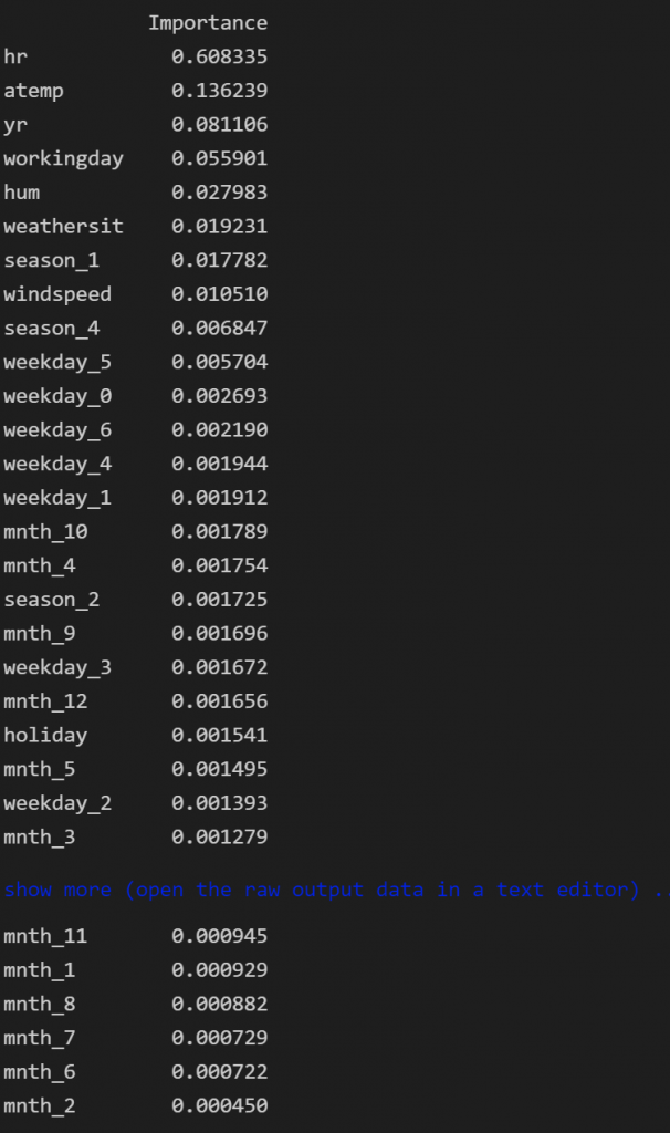
feat_importances = pd.DataFrame(rf.feature_importances_, index=X_train.columns, columns=["Importance"])
feat_importances.sort_values(by='Importance', ascending=False, inplace=True)
feat_importances

feat_importances.plot(kind='bar', figsize=(12,8))

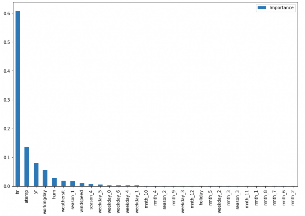
As we can see the most important variables are:

• The Hour with 60%
• The Temperature with14%
• The Year with 8%

Insights

We found that the number of Bike Rentals depends on the hour and the temperature. Also, it seems that there is an interaction between variables, like hour and day of week, or month and year etc and for that reason, the tree-based models like Gradient Boost and Random Forest performed much better than the linear regression. Moreover, the tree-based models are able to capture nonlinear relationships, so for example, the hours and the temperature do not have a linear relationship, so for example, if it is extremely hot or cold then the bike rentals can drop. Our model has an RMSE of 42 in the test dataset which seems to be promising.

Further Analysis

There is always a room of improvement when we build Machine Learning models. For instance we could try the following:

• Transform the cnt column to the logarith of cnt
• Try different models using Grid Search
• Fine tuning of the Hyperparameters of the model

Export the Predictions

# the name of my model is rf - this is how I called it before

# now I re-train my model on the whole dataset
rf = RandomForestRegressor().fit(df.drop('cnt', axis=1), df.cnt)

# I get the predictions
df['Predictions'] = rf.predict(df.drop('cnt', axis=1))

df.to_csv("my_analysis.csv", index=False)